
coresynth ships method-appropriate inference for each estimator, plus a cross-cutting conformal procedure. This article surveys them on a single synthetic panel.
set.seed(123)
N <- 12; TT <- 20; T_pre <- 12
f   <- cumsum(rnorm(TT, 0, 0.5))
lam <- rnorm(N, 1, 0.3)
dat <- expand.grid(time = seq_len(TT), id = paste0("u", seq_len(N)))
dat$y <- as.vector(outer(f, lam)) + rnorm(nrow(dat), 0, 0.3)
dat$d <- as.integer(dat$id == "u1" & dat$time > T_pre)
dat$y[dat$d == 1] <- dat$y[dat$d == 1] + 2.0   # true ATT = 2.0

fit_scm  <- scm_fit(y ~ d | id + time, data = dat, method = "scm")
fit_sdid <- scm_fit(y ~ d | id + time, data = dat, method = "sdid")
fit_gsc  <- scm_fit(y ~ d | id + time, data = dat, method = "gsc", r = 2)
fit_si   <- scm_fit(y ~ d | id + time, data = dat, method = "si")

# The same panel with four treated units, for the routines that resample them
dat4 <- dat
dat4$d <- as.integer(dat4$id %in% c("u1", "u2", "u3", "u4") & dat4$time > T_pre)
dat4$y[dat4$d == 1 & dat4$id != "u1"] <-
  dat4$y[dat4$d == 1 & dat4$id != "u1"] + 2.0
SCM — MSPE ratio permutation test
Abadie et al. (2010). mspe_ratio_pval()
compares the treated unit’s post/pre MSPE ratio against placebo ratios
from every donor. It returns a plain list.
mspe <- mspe_ratio_pval(fit_scm, alternative = "two.sided")
c(p_value = mspe$p_value, ratio_obs = mspe$ratio_obs)
#>    p_value
#> 0.08333333
The returned scm_placebo object has a
plot() method that reproduces the two companion figures of
the paper. type = "gaps" overlays the treated unit’s gap
path (treated minus synthetic control) on the placebo gap paths obtained
by reassigning the intervention to each donor (ADH 2010, Figure 4):
plot(mspe, type = "gaps")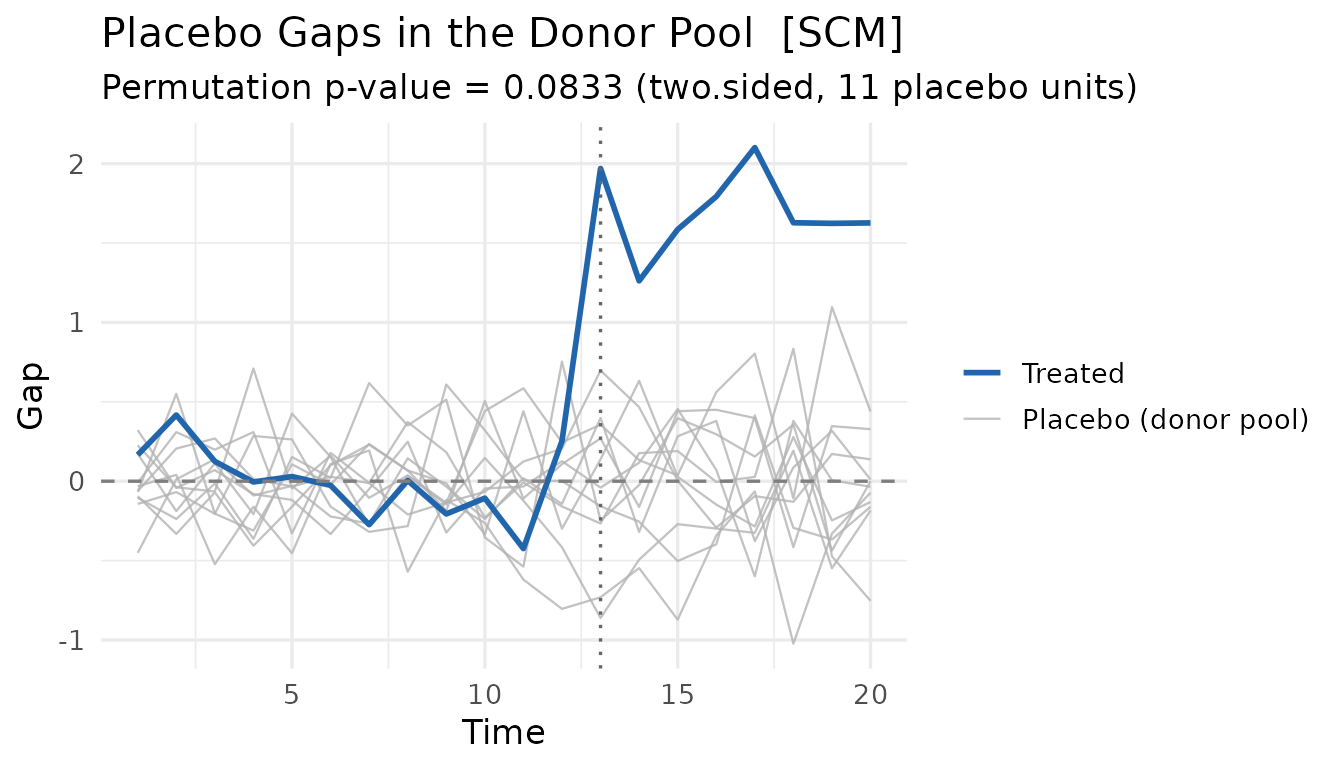
Placebo units whose synthetic control fits poorly before treatment
carry no information about the rarity of a large post-treatment gap; ADH
exclude them with a relative pre-treatment MSPE cutoff (20x/5x/2x in
their Figures 5–7), available here as mspe_prune:
plot(mspe, type = "gaps", mspe_prune = 2)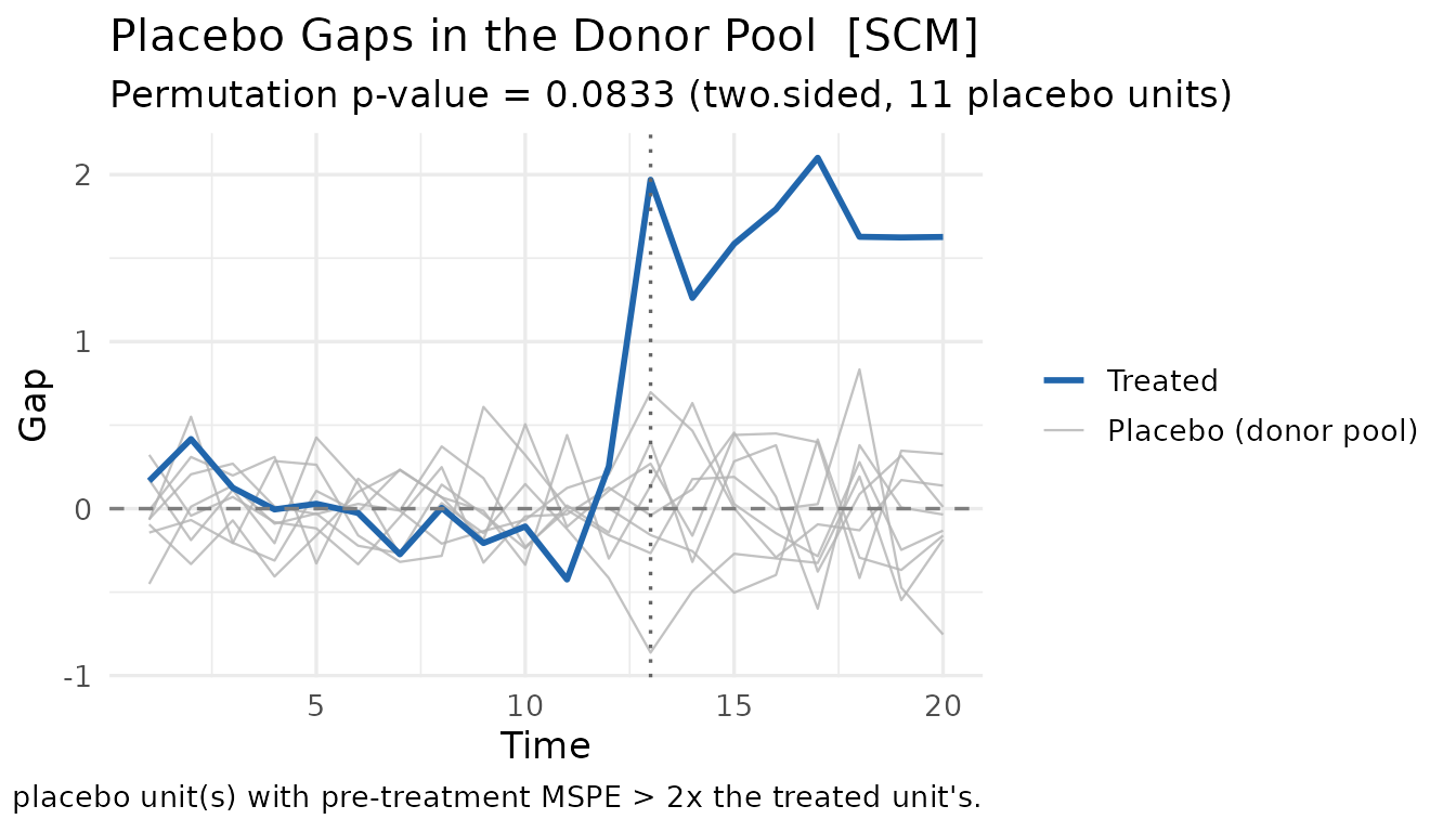
type = "ratios" shows the post/pre-treatment MSPE ratio
of every unit (ADH 2010, Figure 8) — the statistic behind the
permutation p-value, which needs no pruning cutoff by construction:
plot(mspe, type = "ratios")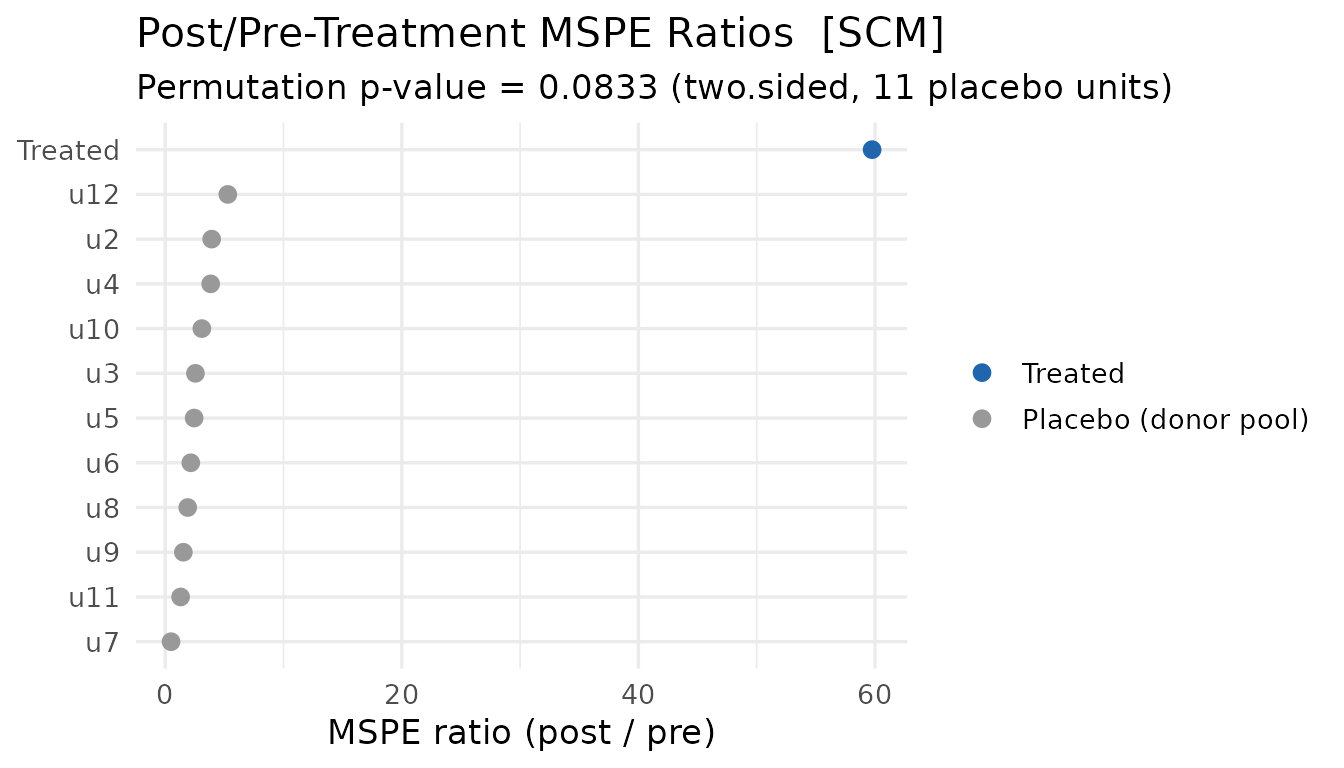
The mspe_prune cutoff applies to the p-value as well as
the picture, and statistic = "post_mspe" ranks the
post-treatment MSPE itself rather than its ratio (Abadie 2021, S.3.5),
which is the variant that needs the cutoff:
mspe_ratio_pval(fit_scm, mspe_prune = 5, statistic = "post_mspe")$p_value
#> [1] 0.08333333
Plotting such a result gives the picture the p-value was computed
from: both views drop the runs the cutoff discarded, and
type = "ratios" draws whichever statistic the test ranked.
Pass mspe_prune = Inf to see every run regardless.
When several units are treated at once the fit pools
them into one synthetic control, and this test no longer applies: the
averaged treated series is less noisy than any single donor, so its MSPE
ratio is inflated and the test over-rejects. Use
scm_rank_pval() instead — the rank-based permutation test
of Abadie & L’Hour (2021, S.3.2), which ranks per-unit statistics so
that only single-unit quantities are ever compared.
For staggered SCM fits, use
scm_inference() — the leave-one-unit-out jackknife
(default) or wild bootstrap of Ben-Michael, Feller & Rothstein
(2022) — described in the Staggered
adoption article. scm_rank_pval() works there too, on a
fit made with pool_cohorts = FALSE.
Series colors, legend text, line types, and the reference lines are
customizable via colors, labels
(e.g. labels = c(treated = "California")),
linetypes
(e.g. linetypes = c(placebo = "dotted")),
vline, and hline — see
?plot.scm_placebo.
SDID — four inference methods
Arkhangelsky et al. (2021); Clarke et al. (2024).
sdid_inference() follows the paper’s three variance
estimators. "bootstrap" (Algorithm 2) draws units with
replacement from the whole panel, treated and control alike, and runs
the whole estimator again on each draw; "jackknife"
(Algorithm 3) drops one unit at a time with the fitted weights held
fixed; "placebo" (Algorithm 4) reassigns the treatment to
control units. The first two need more than one treated unit – the paper
notes the jackknife is not even defined with one – so a single treated
unit calls for "placebo", which assumes the treated and
control units share a noise level. Staggered fits add
"jackknife_global". The result is
broom-friendly.
inf_plac <- sdid_inference(fit_sdid, method = "placebo")

fit_sdid4 <- scm_fit(y ~ d | id + time, data = dat4, method = "sdid")
inf_boot  <- sdid_inference(fit_sdid4, method = "bootstrap", n_boot = 100, seed = 1)

tidy(inf_plac)
#>   term estimate  std.error statistic    p.value conf.low conf.high  method
#> 1  ATT 1.821899 0.09624075  18.93064 0.08333333 1.633271  2.010528 placebo
#>   alternative n_controls staggered
#> 1   two.sided         11     FALSE
tidy(inf_boot)
#>   term estimate std.error statistic      p.value conf.low conf.high    method
#> 1  ATT 1.849042 0.1258999  14.68661 7.854681e-49 1.605685  2.060413 bootstrap
#>   alternative n_controls staggered
#> 1   two.sided          8     FALSE
tidy() returns a one-row data frame with
estimate, std.error, p.value, and
a CI — ready to rbind() into a results table.
glance() gives a compact summary:
glance(inf_boot)
#>      method n_controls staggered estimate std.error      p.value conf.low
#> 1 bootstrap          8     FALSE 1.849042 0.1258999 7.854681e-49 1.605685
#>   conf.high alternative n_boot_valid
#> 1  2.060413   two.sided          100
GSC — parametric and non-parametric
Xu (2017). gsc_boot() is the paper’s parametric
bootstrap (Algorithm 2, sharp fits only), the procedure it proposes when
few units are treated. Each replicate rebuilds the panel without an
effect from the fitted values plus resampled residual series – the
controls’ in-sample residuals, and for the treated units the prediction
errors of control units left out as if they were treated – so its
replicates are draws of the estimation error, and the interval is the
estimate minus their quantiles.
gb <- gsc_boot(fit_gsc, B = 100, alpha = 0.05)
c(ci_lower = gb$ci_lower, ci_upper = gb$ci_upper, p_value = gb$p_value)
#> ci_lower ci_upper  p_value
#> 1.669943 2.324487 0.000000
gsc_inference() resamples units instead: a bootstrap of
the treated and the control units drawn separately, or a jackknife that
drops one unit at a time. Resampling reaches the treated units’ own
noise only through which treated units are drawn, so it needs several of
them; with a single treated unit it stops and points back to
gsc_boot(). On the panel with four treated units:
fit_gsc4 <- scm_fit(y ~ d | id + time, data = dat4, method = "gsc", r = 2)
tidy(gsc_inference(fit_gsc4, method = "jackknife"))
#>   term estimate std.error statistic      p.value conf.low conf.high    method
#> 1  ATT  1.98452 0.1010291  19.64304 6.630308e-86 1.786506  2.182533 jackknife
#>   alternative n_controls staggered
#> 1   two.sided          8     FALSE
SI — bootstrap / jackknife
Agarwal et al. (2025). si_inference() resamples
units in the same way and also handles staggered and multi-arm fits;
each refit keeps the rank k the fit used. For a sharp fit
with one treated unit, use conformal_inference() below.
fit_si4 <- scm_fit(y ~ d | id + time, data = dat4, method = "si")
tidy(si_inference(fit_si4, method = "bootstrap", n_boot = 100, seed = 1))
#>   term estimate  std.error statistic      p.value conf.low conf.high    method
#> 1  ATT 1.992019 0.07726801  25.78065 1.46175e-146 1.870346   2.15603 bootstrap
#>   alternative n_controls staggered
#> 1   two.sided          8     FALSE
Conformal inference (any sharp fit)
Chernozhukov, Wüthrich & Zhu (2021).
conformal_inference() works across scm /
sdid / gsc / mc / si
sharp fits. Under H0: τ = τ0 it re-imputes the treated post-period as
Y1 - τ0, re-estimates the counterfactual on all T
periods, and inverts a moving-block permutation test of the
residuals to get a p-value and a confidence interval.
conf <- conformal_inference(fit_scm, tau0 = 0, level = 0.95)
tidy(conf)
#>   term estimate std.error statistic p.value   conf.low conf.high    method
#> 1  ATT 1.698433        NA        NA     0.1 -0.1072869  3.162241 conformal
#>   alternative n_controls staggered
#> 1   two.sided         11     FALSE
The p-value tests the sharp null τ0 = 0; the CI is obtained by test inversion over a grid. Because the permutation uses |Π| = T cyclic shifts, the smallest attainable p-value is 1/T.
Assembling a results table
Since every inference object tidies to the same columns, comparing
methods is a single rbind():
do.call(rbind, list(
  cbind(method = "sdid (placebo)",   tidy(inf_plac)[c("estimate","p.value","conf.low","conf.high")]),
  cbind(method = "sdid (bootstrap)", tidy(inf_boot)[c("estimate","p.value","conf.low","conf.high")]),
  cbind(method = "scm (conformal)",  tidy(conf)[c("estimate","p.value","conf.low","conf.high")])
))
#>             method estimate      p.value   conf.low conf.high
#> 1   sdid (placebo) 1.821899 8.333333e-02  1.6332710  2.010528
#> 2 sdid (bootstrap) 1.849042 7.854681e-49  1.6056849  2.060413
#> 3  scm (conformal) 1.698433 1.000000e-01 -0.1072869  3.162241