coresynth provides six causal-inference estimators
for panel data behind a single formula interface, with the computational
core (QP solving, SVD, Kalman filtering) written in C++ via
RcppArmadillo. This vignette walks through the basics: fitting a model,
comparing methods, and pulling results out with broom and
plot().
The unified formula
Every estimator is reached through scm_fit() with the
same formula syntax:
outcome ~ treatment | unit_id + time_idThe data must be a long-format balanced panel (one
row per unit–time), and treatment is a 0/1 indicator that
switches on for treated units in post-treatment periods.
method = selects the estimator.
A toy panel
We simulate a balanced panel of 10 units over 20 periods. Unit
u1 is treated from period 11 onward with a true ATT of
2.0.
set.seed(42)
N <- 10; TT <- 20; T_pre <- 10
f   <- cumsum(rnorm(TT, 0, 0.5))     # common factor
lam <- rnorm(N, 1, 0.3)              # unit loadings
dat <- expand.grid(time = seq_len(TT), id = paste0("u", seq_len(N)))
dat$y <- as.vector(outer(f, lam)) + rnorm(nrow(dat), 0, 0.3)
dat$d <- as.integer(dat$id == "u1" & dat$time > T_pre)
dat$y[dat$d == 1] <- dat$y[dat$d == 1] + 2.0   # inject the treatment effect

head(dat)
#>   time id         y d
#> 1    1 u1 0.7590559 0
#> 2    2 u1 0.5774968 0
#> 3    3 u1 0.8414384 0
#> 4    4 u1 0.6355518 0
#> 5    5 u1 1.1532557 0
#> 6    6 u1 0.4384856 0
Fitting one method
fit <- scm_fit(y ~ d | id + time, data = dat, method = "scm")
fit
#> === coresynth fit ===
#> Method : SCM
#> Estimate (ATT): 2.2711
#> Pre-treatment periods: 10
The estimated ATT lives in fit$estimate:
fit$estimate
#> [1] 2.271125
Comparing all six methods
Because the interface is shared, swapping estimators is a one-word change. Here we run all six on the same data (true ATT = 2.0).
methods <- c("scm", "sdid", "gsc", "mc", "tasc", "si")
fits    <- lapply(methods, function(m) scm_fit(y ~ d | id + time, data = dat, method = m))
names(fits) <- methods

data.frame(
  method   = methods,
  estimate = round(sapply(fits, `[[`, "estimate"), 3)
)
#>      method estimate
#> scm     scm    2.271
#> sdid   sdid    2.150
#> gsc     gsc    2.255
#> mc       mc    2.696
#> tasc   tasc    1.154
#> si si 2.346| Method | Full name | Reference |
|---|---|---|
scm |
Synthetic Control Method | Abadie, Diamond & Hainmueller (2010) |
sdid |
Synthetic Difference-in-Differences | Arkhangelsky et al. (2021) |
gsc |
Generalized Synthetic Control | Xu (2017) |
mc |
Matrix Completion | Athey et al. (2021) |
tasc |
Time-Aware Synthetic Control | Rho et al. (2026) |
si |
Synthetic Interventions | Agarwal et al. (2025) |
Visualizing a fit
plot.coresynth() offers three views via
type =.
plot(fits$sdid, type = "trend") # observed vs. synthetic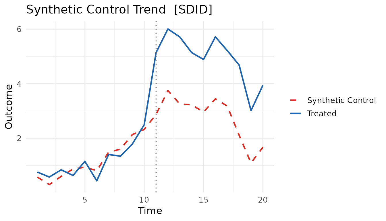
plot(fits$scm, type = "gap") # treatment effect over time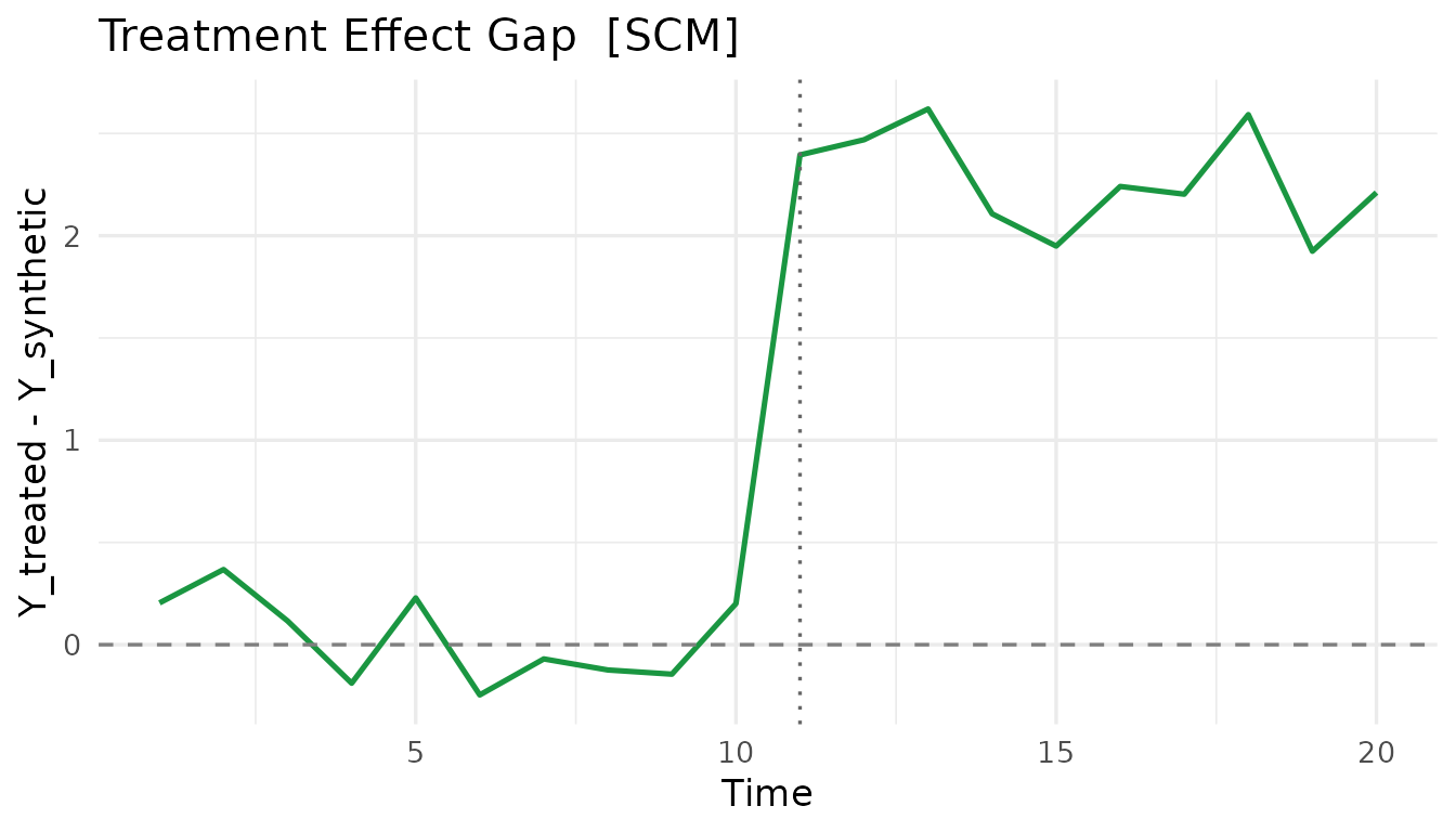
plot(fits$scm, type = "weights") # donor weights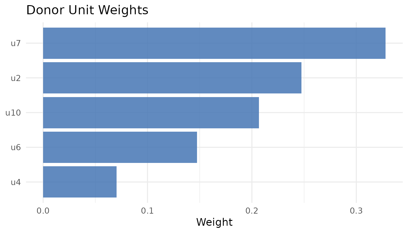
tidy / glance / augment
coresynth integrates with broom, so results drop
straight into tidy workflows and paper tables.
library(broom)

tidy(fits$scm)     # donor weights as a data frame
#>   term   estimate        type
#> 1   u2 0.24752069 unit_weight
#> 2   u3 0.00000000 unit_weight
#> 3   u4 0.07055224 unit_weight
#> 4   u5 0.00000000 unit_weight
#> 5   u6 0.14767482 unit_weight
#> 6   u7 0.32770301 unit_weight
#> 7   u8 0.00000000 unit_weight
#> 8   u9 0.00000000 unit_weight
#> 9  u10 0.20654924 unit_weight
glance(fits$scm)   # one-row model summary
#>   method estimate n_controls n_treated T_pre T_post staggered multi_arm
#> 1    scm 2.271125          9         1    10     10     FALSE     FALSE
For custom plots or diagnostics, the accessor generics return the underlying series from any fit under a uniform interface, whatever the estimation method:
head(treated_outcomes(fits$scm))    # observed treated series
#> [1] 0.7590559 0.5774968 0.8414384 0.6355518 1.1532557 0.4384856
head(synthetic_outcomes(fits$scm))  # estimated counterfactual
#> [1] 0.5549202 0.2098675 0.7254600 0.8242011 0.9246564 0.6843428
dim(donor_outcomes(fits$scm))       # T x N_co donor outcome matrix
#> [1] 20  9
export_json() writes a fit to disk as JSON for
reproducibility or downstream (e.g. AI) workflows:
export_json(fits$scm, file = "scm_result.json")Where to next
- Estimators — covariates, predictors, and method-specific options for all six estimators plus the experimental-design variant.
- Inference — placebo, bootstrap, jackknife, parametric, and conformal inference.
- Staggered adoption — cohort-based estimation when units adopt treatment at different times.