Unified formula interface for Synthetic Control and related causal inference methods. The formula syntax is:
Usage
scm_fit(
  formula,
  data,
  method = c("scm", "sdid", "gsc", "mc", "tasc", "si"),
  predictors = NULL,
  covariates = NULL,
  v_selection = c("insample", "oos"),
  donor_mspe_threshold = Inf,
  lambda_pen = NULL,
  v_optim = c("auto", "coord_descent", "bfgs", "multistart"),
  v_window = NULL,
  nu = NULL,
  fixedeff = FALSE,
  ...
)
Arguments
- formula
A
Formulaobject, e.g.y ~ D | unit + time.- data
A
data.framein long format (one row per unit-time).- method
One of
"scm","sdid","gsc","mc","tasc","si".- predictors
A
list()ofpred()specifications that define the predictor matrix for SCM (see Abadie et al. 2010, S.2.3). Eachpred()entry aggregates one or more variables over a time window. PassNULL(default) to use all pre-treatment outcome periods as predictors; a one-line message states this default when it applies. A specification consisting solely of the outcome variable at each single pre-treatment period (onepred()per period, jointly covering the full pre-treatment window) defines the same predictor matrix and is therefore fitted through the same outcomes-only path asNULL, returning an identical fit; supplyv_optim = "multistart"explicitly to force the predictor-path optimiser instead. Applies tomethod = "scm"only. Predictor rows are scaled by their standard deviation across all units before optimisation, matching the Synth reference implementation (ADH 2011, JSS); passscale_predictors = FALSEto disable.- covariates
An optional named
listof additional time-varying covariates to partial out before estimation. Each element is a character string naming a column indata. Supported formethod = "sdid","scm", and"gsc".- v_selection
V matrix selection method for
method = "scm"."insample"(default) follows Abadie et al. (2010): V is chosen by minimising in-sample pre-treatment MSPE."oos"follows Abadie (2021) S.3.2 / ADH (2015): the pre-treatment window is split into a training half and a validation half. In the default outcomes-as-predictors case, candidate W(V) are fitted on training-half outcomes only, V* minimises the validation-half MSPE, and the final W* is refit with V* on the outcomes of the lastfloor(T_pre/2)pre-treatment periods (sov_weightshasfloor(T_pre/2)entries). With user-suppliedpredictors, the predictor matrix is fixed and only the MSPE evaluation window is restricted to the validation half; lag yourpred()windows to the training period for a fully out-of-sample exercise.- donor_mspe_threshold
Donor pool filtering threshold (Abadie 2021 S.4). For
method = "scm"only. Each donor's individual pre-treatment MSPE (using that donor alone as the counterfactual) is divided by the minimum such MSPE across all donors. Donors whose ratio exceeds this threshold are excluded from estimation.Inf(default) disables filtering.- lambda_pen
Penalised SCM parameter (Abadie & L'Hour 2021, JASA). For
method = "scm"only.NULL(default) runs standard unpenalised SCM."auto"selects the penalty via out-of-sample pre-treatment MSPE on the same validation window asv_selection = "oos". A non-negative number uses that value directly.- v_optim
Outer V-optimisation method for
method = "scm". The outer problem (choose V so that the implied donor weights W(V) minimise pre-treatment outcome MSPE) is non-convex, and a single local search can settle in a poor basin whenpredictorsare supplied."auto"(default) therefore selects"multistart"for predictor-based fits and"coord_descent"for outcomes-only fits (where the single start is empirically reliable)."multistart"runs a deterministic multi-start search: a fixed start set (uniform V, one-hot V per predictor, and 100 fixed-seed random draws) is screened at one inner QP each, the leaders are polished by coordinate descent, and the winner is refined by a Nelder-Mead pass. Its solution is never worse (in pre-treatment loss) than"coord_descent", at roughly the cost of a handful of single-start fits, and is fully reproducible (no RNG state is consumed)."coord_descent"is the classic single-start coordinate descent with an 11-point grid, and is also the outcomes-only and staggered engine and the multi-start never-worse reference."bfgs"(a single-start L-BFGS-B) is deprecated and will be removed in a future release: it has no advantage over"multistart"(which dominates it on predictor fits) or"coord_descent".mspe_ratio_pval()mirrors a multi-start fit in its placebo refits so the permutation test stays symmetric.- v_window
Optional vector of pre-treatment time values (matching the time index in
data) over which the outer V optimisation evaluates the pre-treatment fit, formethod = "scm"(sharp fits only).NULL(default) evaluates on all pre-treatment periods. The window restricts only the outer evaluation loss: predictor matrices (or the full pre-treatment outcome rows in the outcomes-only case) still enter the inner QP unchanged, and the reportedlossandmspe_ratio_pval()MSPE components always cover the full pre-treatment window. Cannot be combined withv_selection = "oos", which manages its own train/validation split.- nu
Partial pooling parameter for staggered SCM fits (Ben-Michael, Feller & Rothstein 2022, JRSS-B).
NULL(default) keeps the per-cohort V-optimised SCM path. A number in[0, 1]switches to partially pooled SCM: all cohort weight vectors are chosen jointly to minimisenu * (normalised pooled pre-treatment imbalance)^2 + (1 - nu) * (normalised per-cohort imbalance)^2, so the aggregate ATT is anchored by the pooled fit.nu = 0is separate per-cohort SCM with uniform lag weights,nu = 1fully pooled, andnu = "auto"uses the paper's heuristic (the ratio of the pooled to the average per-cohort imbalance of the separate solution). The pooled path is outcomes-only and cannot be combined withdonor_mspe_threshold,lambda_pen, orv_selection = "oos". Balance diagnostics are stored infit$pooling. Formethod = "scm"on staggered panels only.- fixedeff
If
TRUE, staggered SCM demeans every unit by its own pre-treatment mean within each cohort before fitting (intercept shift; Ben-Michael, Feller & Rothstein 2022, Section 5.1), which turns the estimator into a weighted difference-in-differences and typically improves fit when outcome levels differ across units. The reportedY_synthis shifted back to the raw outcome scale. Works with both the default and the partially pooled path. Formethod = "scm"on staggered panels only. DefaultFALSE.- ...
Additional arguments forwarded to the specific method (e.g.
r,lambda,zeta2).
Value
An object of classes c("coresynth_<method>", "coresynth").
Fits with staggered adoption additionally inherit from
"coresynth_staggered", and multi-arm SI fits from
"coresynth_multiarm"; S3 methods such as tidy() and augment()
dispatch on these subclasses.
All methods return at minimum:
method: estimator nameestimate: average treatment effect (ATT)times: time index vectorT_pre: number of pre-treatment periodsY_treat: treated unit outcome seriesgap: treatment effect series (Y_treat - counterfactual)
Examples
# Synthetic balanced panel: 10 units over 20 periods, unit 1 treated
# after period 15.
set.seed(1)
panel <- expand.grid(unit = 1:10, year = 1:20)
panel$treated <- as.integer(panel$unit == 1 & panel$year > 15)
panel$gdp <- panel$unit + 0.5 * panel$year +
rnorm(nrow(panel)) + 3 * panel$treated
fit <- scm_fit(gdp ~ treated | unit + year, data = panel, method = "sdid")
summary(fit)
#> === coresynth summary ===
#> Method : SDID
#> Periods : T_pre = 15 | T_post = 5
#> ATT estimate: 3.49975
#> Unit weights (non-zero donors):
#> 2 3 4 5 6 8 9 10
#> 0.0886 0.1557 0.0275 0.1072 0.0966 0.1351 0.1746 0.2147
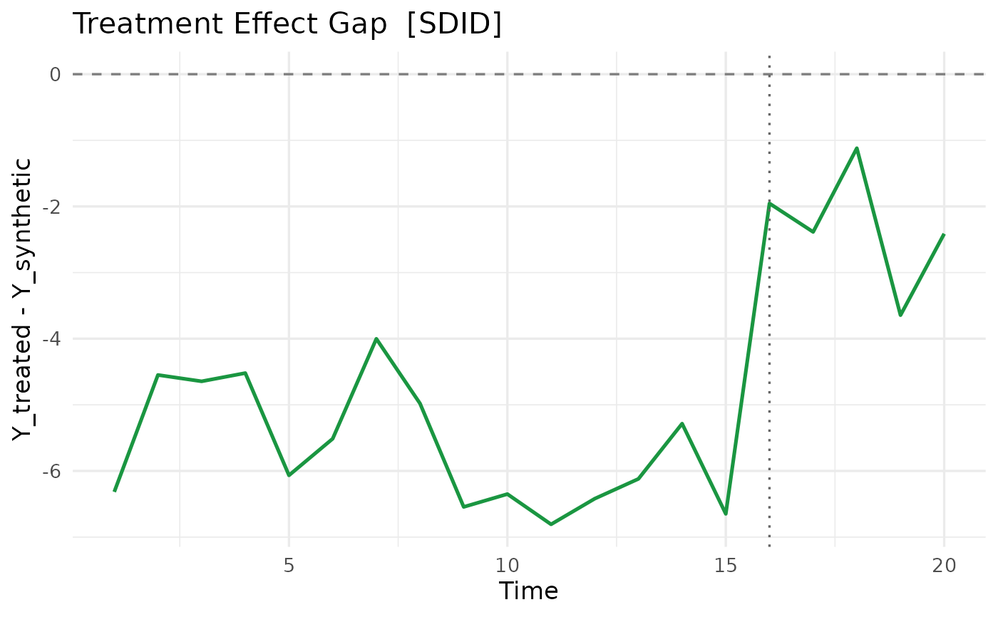
# \donttest{
# Visualise the estimated gap (requires ggplot2)
plot(fit, type = "gap")
 # }
# }