Plot a coresynth model

Usage

# S3 method for class 'coresynth'
plot(
  x,
  type = c("trend", "gap", "weights", "pred_weights"),
  colors = NULL,
  labels = NULL,
  vline = list(),
  vline_offset = 0,
  hline = list(),
  fill = NULL,
  top_n = Inf,
  align = FALSE,
  show_donors = 0,
  ...
)

Arguments

x: A coresynth object.
type: One of "trend" (observed vs synthetic), "gap" (ATT over time), "weights" (donor unit weight bar chart; SDID fits get a second panel with the time weight profile), or "pred_weights" (the predictor/variable weight matrix \(V\) as a bar chart; sharp SCM only).
colors: For type = "trend": a named vector overriding series colors, e.g. c(treated = "black") (valid keys: "treated", "synthetic", plus "donors" when show_donors > 0). For type = "gap": a single color string for the gap line. Ignored for type = "weights" (use fill instead).
labels: For type = "trend": a named vector overriding the legend text of individual series, e.g. c(treated = "California") (valid keys: "treated", "synthetic", plus "donors" when show_donors > 0). Series not mentioned keep their default label; colors and labels address series by the same keys, independent of the displayed legend text. Ignored for other types (no legend).
vline: Aesthetic overrides for the vertical treatment-time line, as a list passed to ggplot2::geom_vline() (e.g. list(color = "red")). NULL or FALSE hides the line entirely. The list may also carry an xintercept element giving one or more absolute positions on the time axis (e.g. list(xintercept = 1988), or a date string such as "1989-01-01" on a Date axis), replacing the default treatment-time position; for placement relative to the treatment period use vline_offset instead. Applies to "trend" and "gap".
vline_offset: For type = "trend" and "gap": where to draw the vertical treatment line, in periods relative to the first post-treatment period. The default 0 keeps the line at the first post-treatment period; -1 moves it to the last pre-treatment period, and fractional values interpolate between adjacent observed times (-0.5 is midway between the last pre- and first post-treatment period), which works on numeric, Date, and POSIXct axes alike. Cannot be combined with an xintercept element in vline.
hline: Aesthetic overrides for the horizontal zero line in type = "gap", as a list passed to ggplot2::geom_hline(). NULL or FALSE hides the line. Ignored for other types.
fill: For type = "weights" and type = "pred_weights": a single color string overriding the bar fill. Ignored for other types.
top_n: For type = "weights": show only the top_n donors with the largest weights (default Inf keeps every donor with a non-negligible weight). For type = "pred_weights": show only the top_n predictors with the largest \(V\) weights (default Inf shows every predictor). Ignored for other types (and for the SDID time weight panel, which is always shown in full).
align: For type = "trend" and "gap": when TRUE, shift the synthetic series by its pre-treatment level gap to the treated series so that both are drawn on the same level. SDID matches trends only up to a free intercept, so its raw trend plot shows the synthetic control at a different level; with align = TRUE the offset is the time-weighted (\(\lambda\)) pre-period gap, which makes the average post-period gap in the plot equal the SDID estimate exactly. Other methods use the plain pre-period mean gap (usually a negligible shift, since they already match levels). Default FALSE (raw series).
show_donors: For type = "trend": also draw the outcome paths of the show_donors donor units with the largest weights as thin background lines (Inf shows every donor). Requires a fit that stores donor unit weights and outcomes (sharp SCM/SDID/SI). Default 0 (no donor paths).
...: Ignored.

Value

A ggplot2 plot object.

Examples

set.seed(1)
panel <- expand.grid(unit = 1:10, year = 1:20)
panel$treated <- as.integer(panel$unit == 5 & panel$year > 15)
panel$gdp <- panel$unit + 0.5 * panel$year +
  rnorm(nrow(panel)) + 3 * panel$treated
fit <- scm_fit(gdp ~ treated | unit + year, data = panel, method = "scm")
#> predictors = NULL: using the outcome in each of the 15 pre-treatment periods as predictors (outcomes-only SCM).

# \donttest{
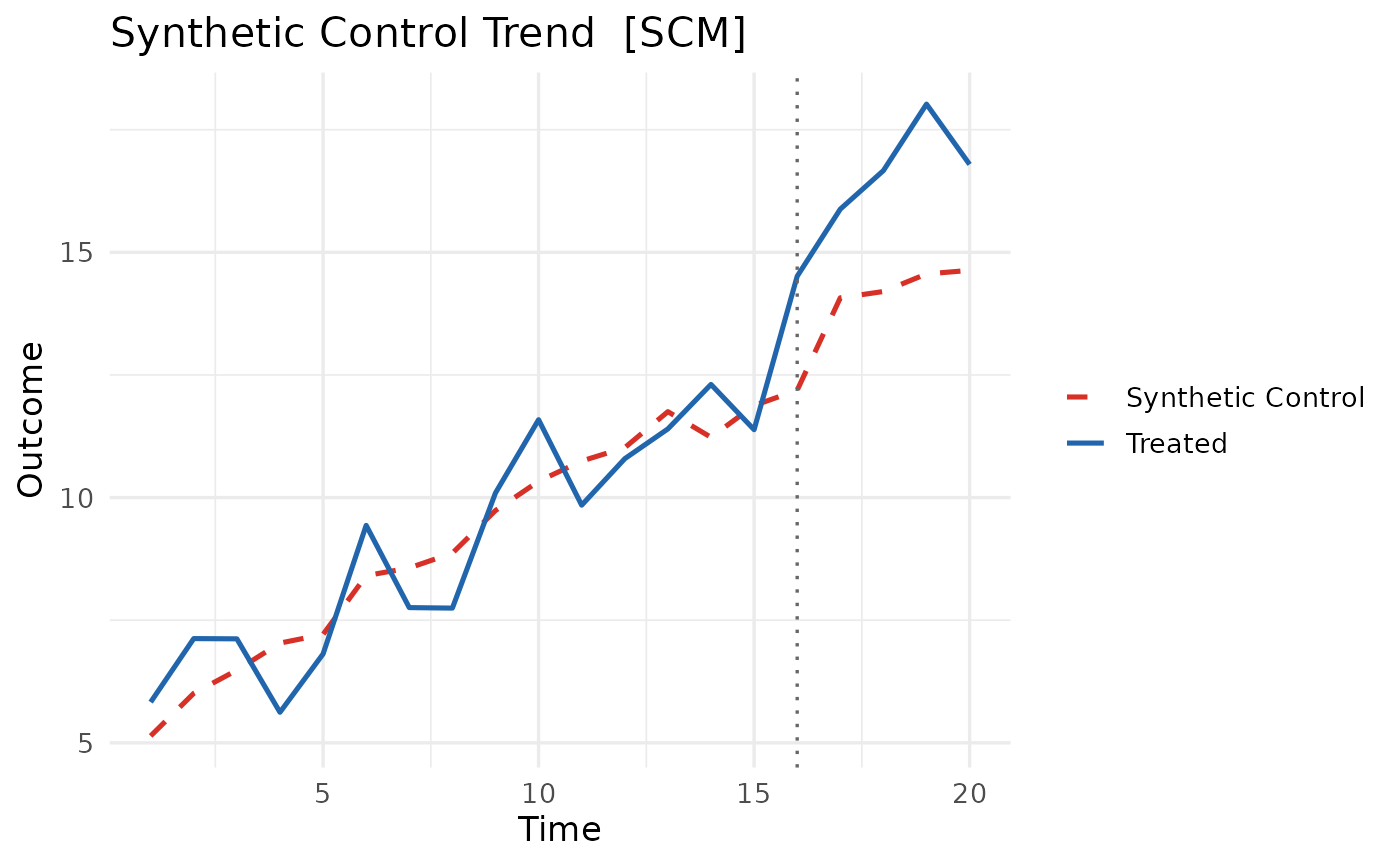
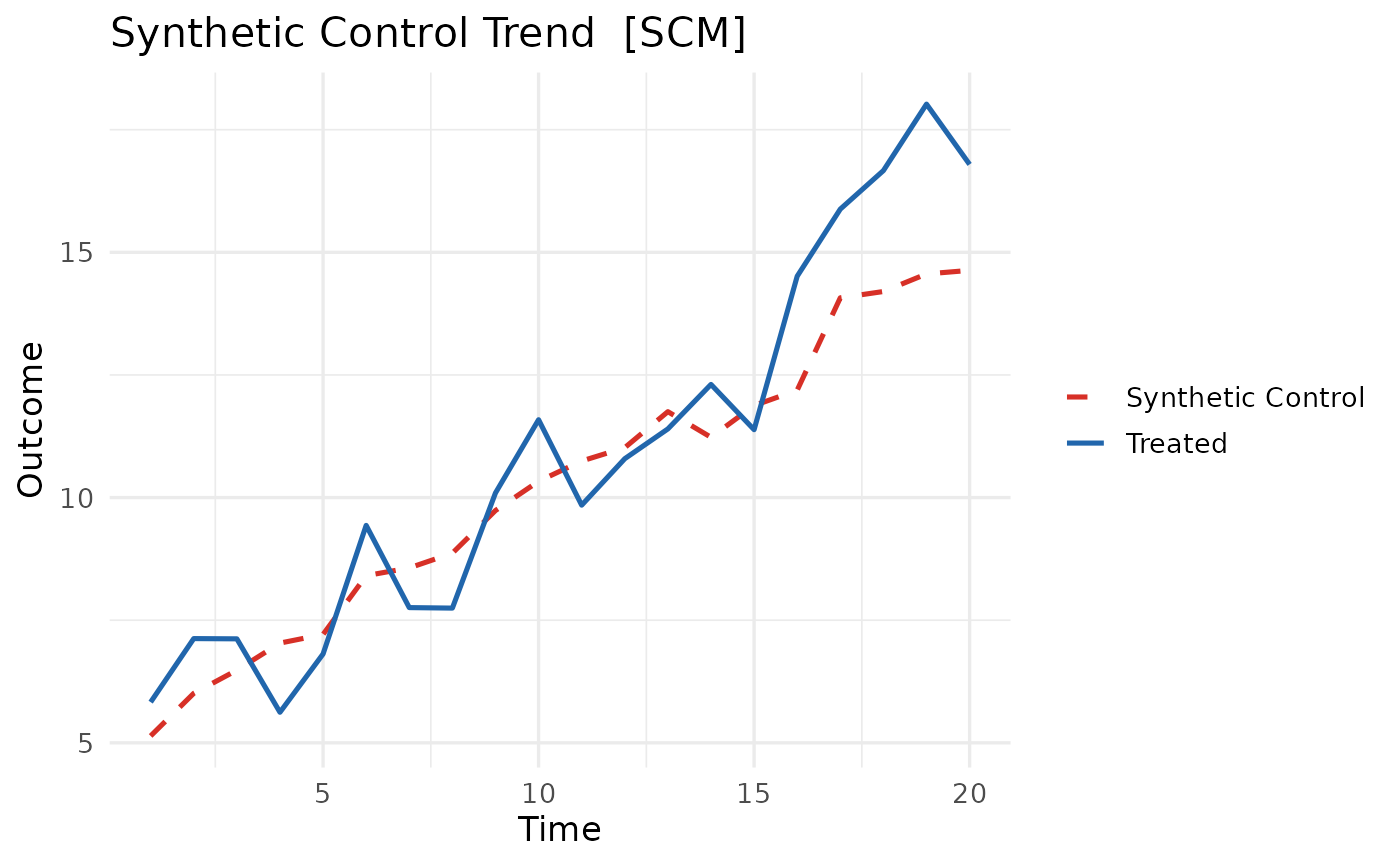
plot(fit, type = "trend")

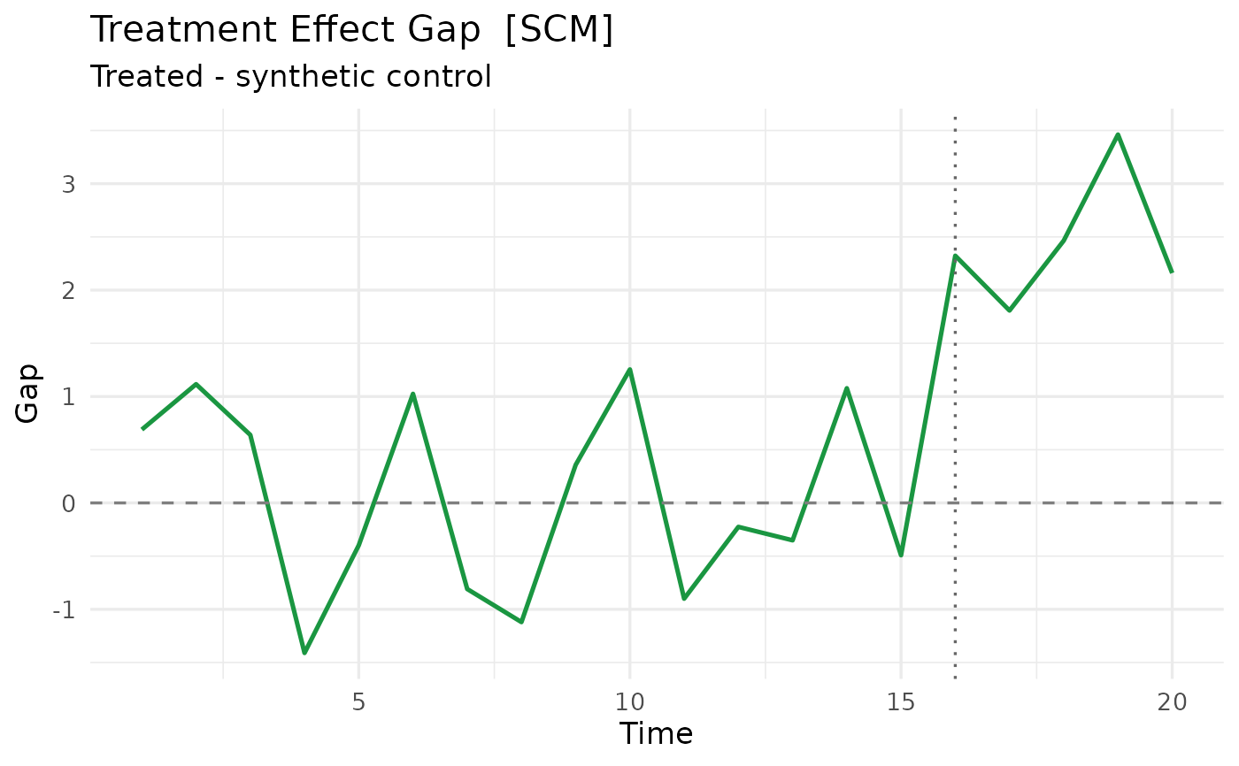
plot(fit, type = "gap")

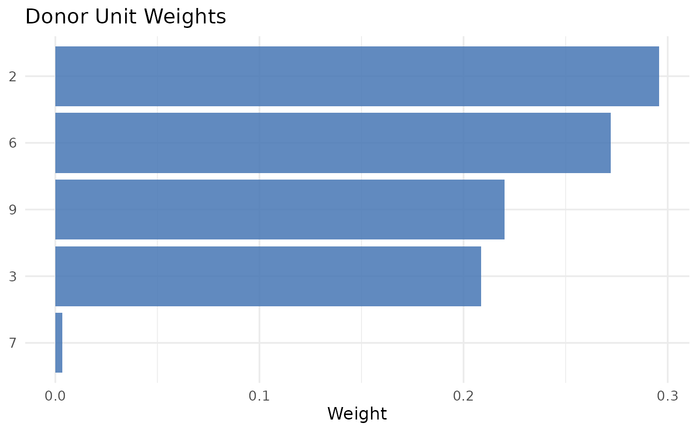
plot(fit, type = "weights")

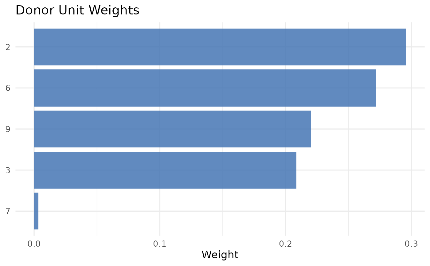plot(fit, type = "weights", top_n = 5)


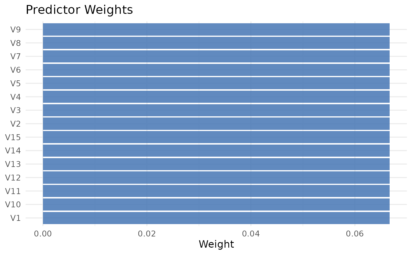
# Predictor (V) weights: which predictors the fit leans on
plot(fit, type = "pred_weights")


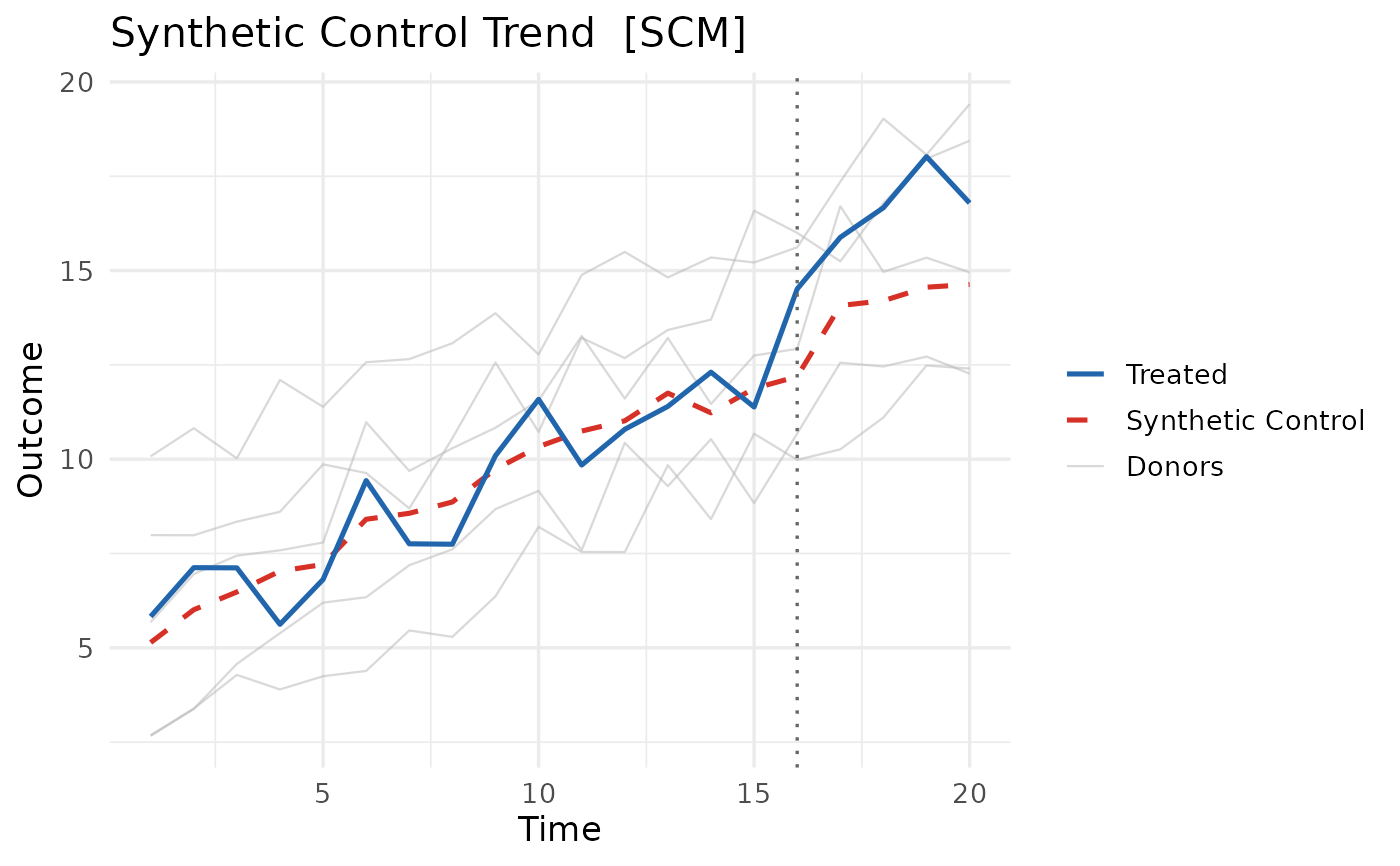
# Overlay the five largest donors behind the treated/synthetic series
plot(fit, type = "trend", show_donors = 5)


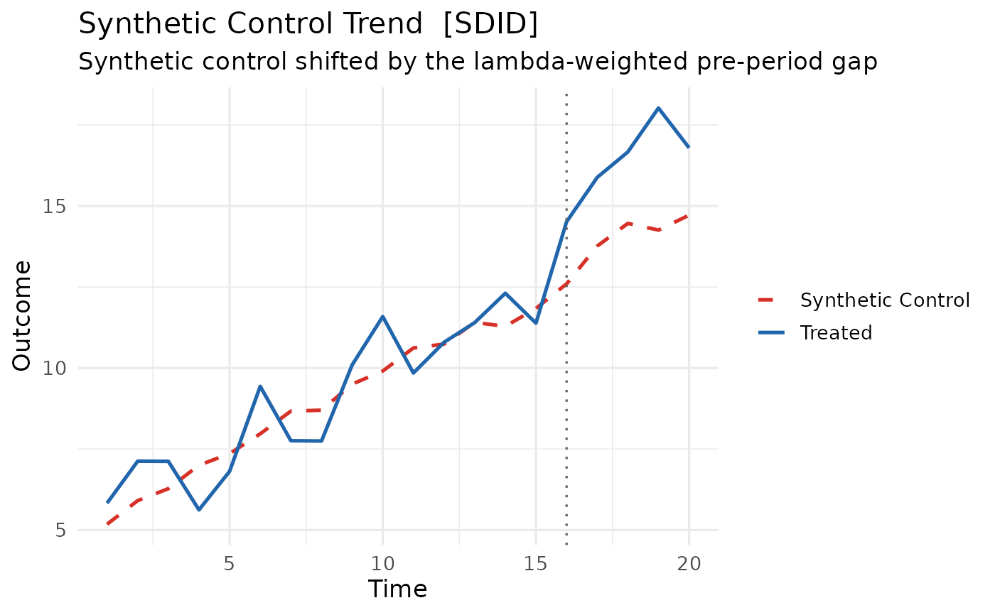
# SDID: align the synthetic series on the lambda-weighted pre-period level
fit_sdid <- scm_fit(gdp ~ treated | unit + year, data = panel, method = "sdid")
plot(fit_sdid, type = "trend", align = TRUE)

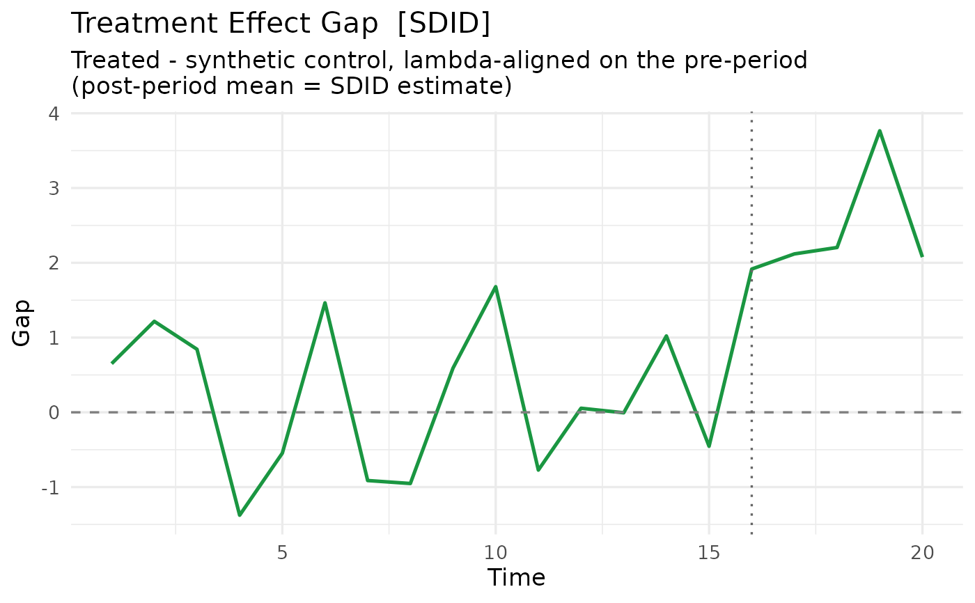
plot(fit_sdid, type = "gap",   align = TRUE)


# Customize series colors, legend text, and reference lines
plot(fit, type = "trend",
     colors = c(treated = "black"),
     labels = c(treated = "Unit 5"),
     vline  = list(color = "red", linetype = "dashed"))


# Move the treatment line one period earlier (last pre-treatment period),
# pin it to an absolute time, or drop it entirely
plot(fit, type = "trend", vline_offset = -1)

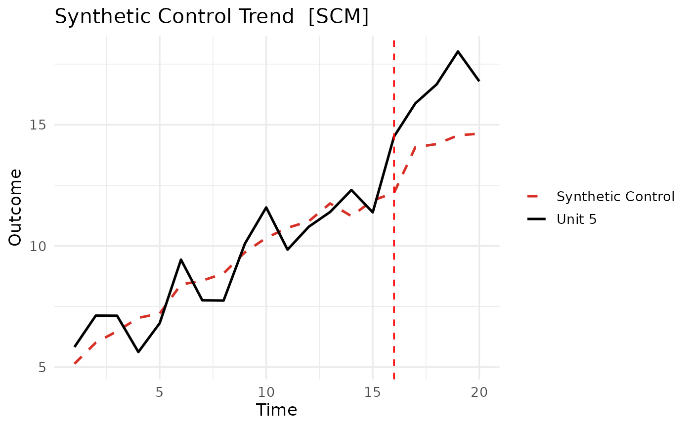
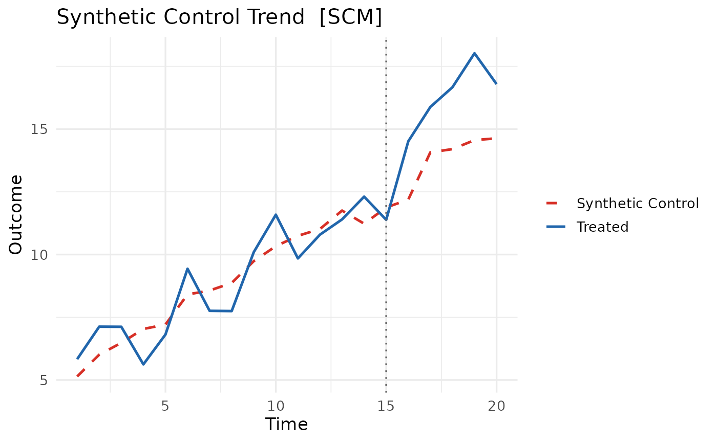
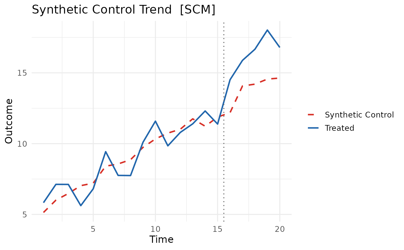
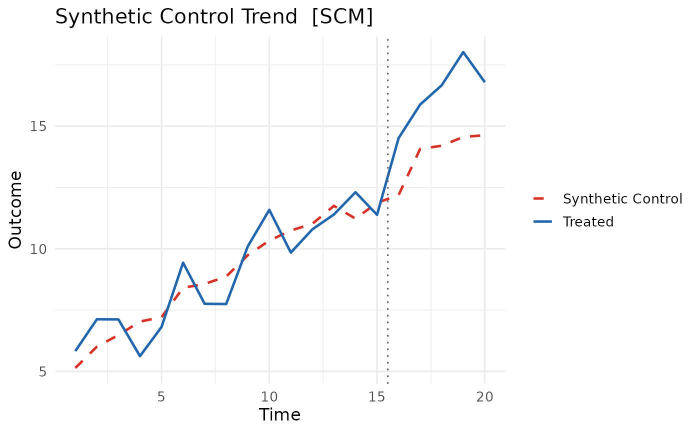
plot(fit, type = "trend", vline = list(xintercept = 15.5))

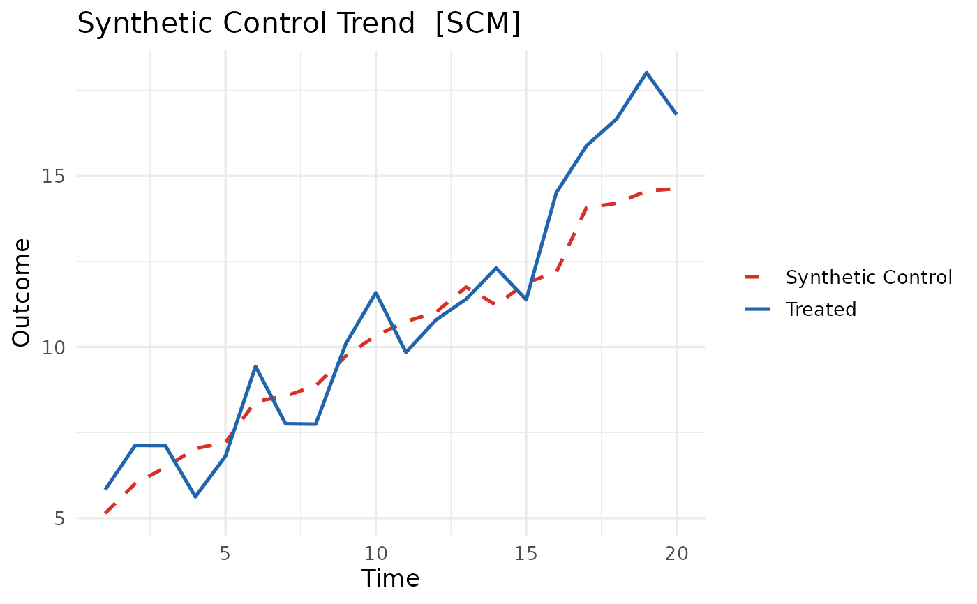
plot(fit, type = "trend", vline = FALSE)

# }