
coresynth is a high-performance R package that provides six causal inference methods for panel data through a unified formula interface. All core optimizations (QP solving, SVD, Kalman filtering) are implemented in C++ via RcppArmadillo, so estimation stays fast even on larger donor pools (see the Performance section for timings).
Installation
# From CRAN
install.packages("coresynth")

# Development version from GitHub
pak::pak("yo5uke/coresynth")
Quick Start
coresynth fits causal panel models through a single formula interface, y ~ d | id + time. This section walks through the classic Synthetic Control Method (SCM); the same formula works for five other methods (see Supported Methods).
Your data should be a balanced panel in long format (one row per unit × time), with:
-
y— the outcome variable -
d— the treatment indicator:0normally,1for a treated unit in periods at or after its treatment starts -
id— the unit identifier -
time— the time identifier
library(coresynth)

# Generate a balanced panel (10 units, 20 periods, true ATT = 2.0)
set.seed(42)
N <- 10; TT <- 20; T_pre <- 10
f   <- cumsum(rnorm(TT, 0, 0.5))
lam <- rnorm(N, 1, 0.3)
dat <- expand.grid(time = seq_len(TT), id = paste0("u", seq_len(N)))
dat$y <- as.vector(outer(f, lam)) + rnorm(nrow(dat), 0, 0.3)
dat$d <- as.integer(dat$id == "u1" & dat$time > T_pre)   # u1 treated from t=11 on
dat$y[dat$d == 1] <- dat$y[dat$d == 1] + 2.0              # true ATT = 2

fit_scm <- scm_fit(y ~ d | id + time, data = dat, method = "scm")
summary(fit_scm)
#> === coresynth summary ===
#> Method : SCM
#> Periods : T_pre = 10 | T_post = 10
#> ATT estimate: 2.271125
#> Unit weights (non-zero donors):
#>     u2     u4     u6     u7    u10
#> 0.2475 0.0706 0.1477 0.3277 0.2065
The key arguments of scm_fit():
-
formula—y ~ d | id + time, matching the columns above -
data— the long-format panel -
method— the estimator to use ("scm","sdid","gsc","mc","tasc", or"si"); all take the same formula
Many more arguments are available for covariate adjustment, donor selection, and staggered adoption — see the Covariates and Staggered Adoption sections below, or ?scm_fit.
# Observed vs. synthetic trend
plot(fit_scm, type = "trend")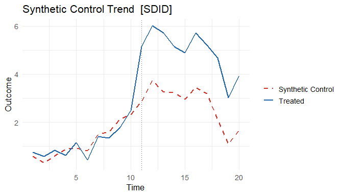
# Treatment effect over time
plot(fit_scm, type = "gap")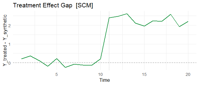
# Donor unit weights
plot(fit_scm, type = "weights")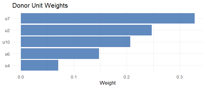
Supported Methods
The same formula and data work for all six methods — just change method:
methods <- c("scm", "sdid", "gsc", "mc", "tasc", "si")
fits    <- lapply(methods, \(m) scm_fit(y ~ d | id + time, data = dat, method = m))
names(fits) <- methods

# Compare ATT estimates (true value = 2.0)
data.frame(
  method   = methods,
  estimate = round(sapply(fits, `[[`, "estimate"), 3)
)
#>      method estimate
#> scm     scm    2.271
#> sdid   sdid    2.150
#> gsc     gsc    2.255
#> mc       mc    2.696
#> tasc   tasc    1.154
#> si si 2.346| Method | Full name | Reference | Treatment | Covariates | Inference |
|---|---|---|---|---|---|
scm |
Synthetic Control Method | Abadie, Diamond & Hainmueller (2010); staggered: Ben-Michael, Feller & Rothstein (2022) | Sharp & Staggered |
pred() list |
mspe_ratio_pval(), scm_inference(), conformal_inference()
|
sdid |
Synthetic Difference-in-Differences | Arkhangelsky et al. (2021) | Sharp & Staggered | covariates= |
sdid_inference(), conformal_inference()
|
gsc |
Generalized Synthetic Control | Xu (2017) | Sharp & Staggered |
covariates= time-varying |
gsc_boot(), gsc_inference(), conformal_inference()
|
mc |
Matrix Completion | Athey et al. (2021) | Sharp & Staggered | — | conformal_inference() |
tasc |
Time-Aware Synthetic Control | Rho et al. (2026) | Sharp & Staggered | — | — |
si |
Synthetic Interventions | Agarwal et al. (2025) | Sharp, Staggered & Multi-arm | — |
si_inference(), conformal_inference()
|
conformal_inference() (Chernozhukov, Wüthrich & Zhu 2021) provides permutation-based p-values and confidence intervals for sharp fits across scm/sdid/gsc/mc/si.
Staggered Adoption
All six methods support staggered adoption using a cohort-based approach (Clarke et al. 2023): each adoption cohort is fitted separately and the cohort ATTs are aggregated with weights proportional to N_treated × T_post.
# u1: treated from t=11, u2: treated from t=16
dat_s        <- dat
dat_s$d      <- 0L
dat_s$d[dat_s$id == "u1" & dat_s$time > 10] <- 1L
dat_s$d[dat_s$id == "u2" & dat_s$time > 15] <- 1L
dat_s$y[dat_s$d == 1] <- dat_s$y[dat_s$d == 1] + 2.0

# All methods detect staggered timing automatically
fit_sdid <- scm_fit(y ~ d | id + time, data = dat_s, method = "sdid")
fit_gsc  <- scm_fit(y ~ d | id + time, data = dat_s, method = "gsc")
fit_mc   <- scm_fit(y ~ d | id + time, data = dat_s, method = "mc")
fit_si   <- scm_fit(y ~ d | id + time, data = dat_s, method = "si")

# Cohort-level estimates are accessible
fit_sdid$cohort_estimates
#>   cohort estimate weight n_treated T_pre T_post
#> 1     11    1.97  0.667         1    10      9
#> 2     16    2.03  0.333         1    10      4

# control_group = "clean" (default) uses never-treated + future-adopters as donors
# control_group = "never_treated" restricts to never-treated only
fit_sdid_clean <- scm_fit(y ~ d | id + time, data = dat_s, method = "sdid",
                          control_group = "never_treated")
SCM: Partially Pooled Synthetic Controls
The original SCM targets a single treated unit, so its staggered extension deserves a note. coresynth follows Ben-Michael, Feller & Rothstein (2022): units adopting at the same time are averaged into one cohort (fully pooling within a cohort is justified by their theory, since the data-generating process cannot vary across units sharing one adoption time), and each cohort is matched to its own synthetic control before aggregation. Two arguments control how the cohort fits interact:
# nu in [0, 1] trades off per-cohort fit (nu = 0) against the fit of the
# *average* placebo gap across cohorts (nu = 1), which anchors the aggregate
# ATT. nu = "auto" uses the paper's heuristic.
fit_pp <- scm_fit(y ~ d | id + time, data = dat_s, method = "scm",
                  nu = "auto", fixedeff = TRUE)
fit_pp$pooling   # balance diagnostics: q_sep / q_pool vs. separate SCM

# fixedeff = TRUE demeans each unit by its own pre-treatment mean
# (an intercept shift), helpful when outcome levels differ across units.

# Wild bootstrap inference (weights held fixed, multiplier resampling)
scm_inference(fit_pp, n_boot = 1000, seed = 1)
With nu = NULL (default) each cohort is fitted independently with the classic V-optimised SCM, which reproduces the behaviour of earlier versions.
Covariates
SCM: Predictor Variables via pred()
SCM supports covariate-based matching following Abadie et al. (2010) S.2.3. Use pred(vars, times, op) to specify which variables and time windows to include in the predictor matrix:
# Assume dat has extra columns: income, unemp
fit_scm_cov <- scm_fit(
  y ~ d | id + time,
  data   = dat,
  method = "scm",
  predictors = list(
    pred(c("income", "unemp"), 1:8),   # average income & unemp over pre-period
    pred("y", 5),                       # outcome at a specific pre-treatment year
    pred("y", 1:4, op = "mean")         # outcome averaged over early pre-period
  )
)
summary(fit_scm_cov)   # shows predictor balance table
Each pred() call aggregates one or more variables over a time window using op = "mean" (default), "median", or "sum". Multiple pred() calls with different windows can be combined freely in the list.
GSC: Time-Varying Covariates
GSC supports time-varying covariate adjustment via the full EM algorithm of Xu (2017). Pass a character vector of column names as covariates:
# Assume dat has a time-varying column: gdp_growth
fit_gsc_cov <- scm_fit(
  y ~ d | id + time,
  data       = dat,
  method     = "gsc",
  r          = 2,
  covariates = "gdp_growth"
)
fit_gsc_cov$beta   # estimated beta coefficient(s)
The EM loop alternates between:
- E-step: SVD of to update factors ,
- M-step: Ridge OLS of residuals on to update
Treated unit loadings are estimated from covariate-demeaned pre-treatment data per Xu (2017) Step 2. When covariates = NULL (default), the plain 3-step SVD estimator () is used.
Inference
SCM: In-Space Placebo Test
mspe_ratio_pval() runs the in-space placebo study of Abadie, Diamond & Hainmueller (2010): the intervention is reassigned to each donor unit and the treated unit’s post/pre-treatment MSPE ratio is compared against the placebo distribution. The result can be plotted directly.
scm_p <- mspe_ratio_pval(fits$scm)
scm_p$p_value
#> [1] 0.1

# Treated gap vs. placebo gaps in the donor pool (ADH 2010, Figures 4-7)
plot(scm_p, type = "gaps")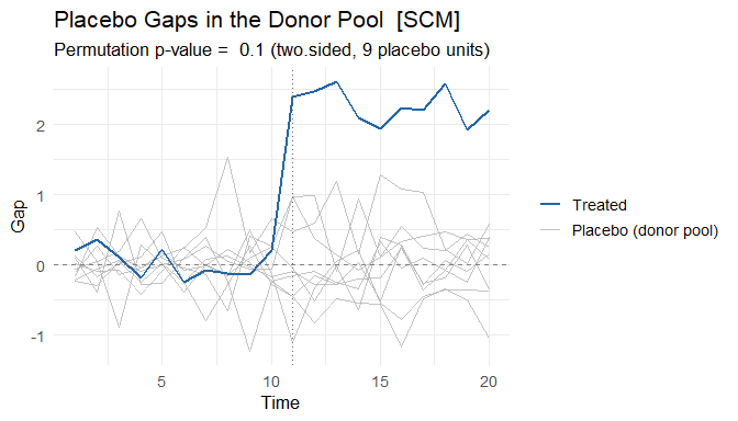
Placebo units with a poor pre-treatment fit can be pruned with mspe_prune (e.g. plot(scm_p, type = "gaps", mspe_prune = 5) excludes units whose pre-treatment MSPE exceeds 5 times the treated unit’s).
# Post/pre-treatment MSPE ratio of every unit (ADH 2010, Figure 8)
plot(scm_p, type = "ratios")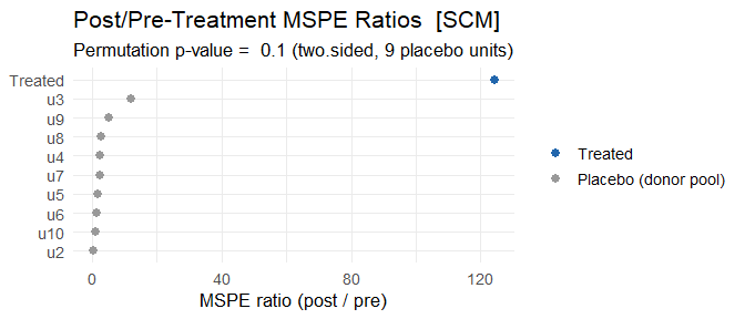
Other Inference Methods
# SDID: four inference methods — placebo, bootstrap, jackknife, jackknife_global
sdid_inf <- sdid_inference(fits$sdid, method = "placebo")
tidy(sdid_inf)   # broom-style one-row data.frame

sdid_boot <- sdid_inference(fits$sdid, method = "bootstrap", n_boot = 200, seed = 1)
tidy(sdid_boot)

# GSC: parametric bootstrap under H0 (sharp only)
gsc_ci <- gsc_boot(fits$gsc, B = 200, alpha = 0.05)
cat("95% CI: [", gsc_ci$ci_lower, ",", gsc_ci$ci_upper, "]\n")

# GSC / SI: non-parametric inference (sharp + staggered)
gsc_inf <- gsc_inference(fits$gsc, method = "jackknife")
si_inf  <- si_inference(fits$si,  method = "bootstrap", n_boot = 200, seed = 1)
tidy(gsc_inf)
tidy(si_inf)

# Conformal inference (Chernozhukov, Wüthrich & Zhu 2021) — sharp fits for
# scm / sdid / gsc / mc / si. Re-estimates the counterfactual under the null
# and inverts a moving-block permutation test for a p-value and CI.
conf <- conformal_inference(fits$scm, tau0 = 0, level = 0.95)
tidy(conf)
tidyverse / broom Integration
library(broom)

# Extract weights as a data frame
tidy(fits$scm)

# Summary row
glance(fits$scm)

# JSON export (for reproducibility and AI workflows)
export_json(fits$scm, file = "scm_result.json")
Every plot() view also has a matching data extractor. plot_data() returns the tidy data frame that a figure is drawn from — taking the same type argument as plot() — so you can rename the simplified series labels, drop the numbers into a table, or build a bespoke figure with your own code. plot() stays the quick path; plot_data() is the handle when you want the data itself. For example, the "trend" view:
Performance
On a 100-donor, 10-year monthly panel, a full SCM fit and its in-space placebo test across all 100 donors both complete in well under a second; Synth takes about a minute and a half for the fit alone, and roughly two hours for the placebo test, on the same data and predictor specification (outcomes-only, matching solutions). Measured against Synth 1.1.10 on Windows 11 / R 4.6.1.
| Panel | Synth fit | coresynth fit | Synth placebo (all donors) | coresynth placebo (all donors) |
|---|---|---|---|---|
| 40 donors, 2 yr pre / 5 mo post | 6.8 s | 3 ms | 4.2 min | 10 ms |
| 100 donors, 8 yr pre / 2 yr post (monthly) | 81 s | 30 ms | ~115 min | 0.3 s |
References
- Abadie, A., Diamond, A., & Hainmueller, J. (2010). Synthetic control methods for comparative case studies. JASA, 105(490), 493–505.
- Agarwal, A., Shah, D., & Shen, D. (2025). Synthetic interventions: extending synthetic controls to multiple treatments. Operations Research. doi:10.1287/opre.2025.1590
- Arkhangelsky, D., Athey, S., Hirshberg, D. A., Imbens, G. W., & Wager, S. (2021). Synthetic difference-in-differences. AER, 111(12), 4088–4118.
- Ben-Michael, E., Feller, A., & Rothstein, J. (2022). Synthetic controls with staggered adoption. JRSS-B, 84(2), 351–381.
- Athey, S., Bayati, M., Doudchenko, N., Imbens, G., & Khosravi, K. (2021). Matrix completion methods for causal panel data models. JASA, 116(536), 1716–1730.
- Chernozhukov, V., Wüthrich, K., & Zhu, Y. (2021). An exact and robust conformal inference method for counterfactual and synthetic controls. JASA, 116(536), 1849–1864.
- Rho, H., et al. (2026). Time-aware synthetic control. Working paper.
- Xu, Y. (2017). Generalized synthetic control method. Political Analysis, 25(1), 57–76.