Implementing Synthetic Difference-in-Differences in R with {coresynth}

Introduction

The {coresynth} package is an R package I developed to implement methods related to the synthetic control method easily and quickly, including the Synthetic Control Method (SCM), Synthetic Difference-in-Differences (SDID), Generalized Synthetic Control (GSC), and Matrix Completion (MC). While the previous post covered the basic synthetic control method, this post focuses on Synthetic Difference-in-Differences (SDID), walking step-by-step from an overview of the method to model estimation, visualization, and inference procedures using coresynth.

What is Synthetic Difference-in-Differences?

Proposed by Arkhangelsky et al. (2021) in the American Economic Review, Synthetic Difference-in-Differences is an important method in causal inference. SDID combines two of the most widely used empirical methodologies in econometrics: Difference-in-Differences (DID) and the Synthetic Control Method (SCM) (Abadie et al. 2010).

Traditional DID relies on the parallel trends assumption, positing that in the absence of treatment, the average outcomes of the treated and control units would have moved in parallel over time. In practice, this assumption often fails when treated and untreated units differ substantially in their observable and unobservable characteristics. Standard DID also assigns uniform weights to all control units and all pre-treatment periods, regardless of how relevant they are for predicting the treated trajectory.

On the other hand, SCM constructs a data-driven weighted average of control units (unit weights $\omega_i$) to reproduce the treated unit’s pre-treatment outcome levels. However, standard SCM does not incorporate an intercept shift (fixed effects) and restricts weights to the simplex ($\sum \omega_i = 1, \omega_i \ge 0$). As a result, when the treated unit lies outside the convex hull of the donor pool (for example, when the treated unit has a consistently higher baseline level than any donor), SCM cannot extrapolate, which can cause poor pre-treatment fit and bias.

SDID synthesizes the core strengths of both worlds by introducing three complementary mechanisms:

Unit weights ($\hat\omega_i$): Control units are reweighted so that their weighted average exhibits parallel trends with the treated unit prior to intervention, relaxing the traditional DID requirement that all controls be parallel on average.
Time weights ($\hat\lambda_t$): Pre-treatment periods are reweighted so that recent pre-treatment periods matching the post-treatment counterfactual slope receive greater emphasis, making the estimator robust to time-varying confounders.
Double differencing (Intercept shift): Like DID, SDID incorporates unit and time fixed effects, absorbing permanent level differences between the treated unit and the donor pool.

Mathematically, the SDID treatment effect for a single treated unit is expressed as:

\[\hat{\tau}^{\text{sdid}} = \left( \bar{Y}_{\text{post}}^{\text{tr}} - \sum_{t=1}^{T_{\text{pre}}} \hat{\lambda}_t Y_{1t} \right) - \sum_{i \in \text{control}} \hat{\omega}_i \left( \bar{Y}_{\text{post}, i} - \sum_{t=1}^{T_{\text{pre}}} \hat{\lambda}_t Y_{it} \right)\]

where $\bar{Y}_{\text{post}}^{\text{tr}}$ is the post-treatment average of the treated unit, $Y_{1t}$ is the treated unit’s outcome at pre-treatment time $t$, and $\bar{Y}_{\text{post}, i}$ is the post-treatment average of control unit $i$.

Why Use {coresynth} for SDID?

While {synthdid} is widely considered the standard R package for SDID, empirical causal inference frequently requires repeated computations: calculating standard errors via bootstrap, running leave-one-out placebo tests across dozens of donors, conducting sensitivity analyses, or testing multiple treatment specifications.

The {coresynth} package is designed and implemented in C++ via RcppArmadillo to enable fast analysis without sacrificing mathematical precision:

⚡ Fast Coordinate Descent & Factor-Form Solvers: In coresynth 1.0.0 and above, SDID unit weights are computed directly in factor form rather than forming and decomposing the dense $N \times N$ donor Gram matrix. This makes estimation and inference routines 5–10× faster on panels with many donors.
🧩 Unified Interface: Run SDID alongside SCM, Generalized Synthetic Control (GSC), Matrix Completion (MC), Time-Aware Synthetic Control (TASC), and Synthetic Interventions (SI) through the exact same scm_fit() formula syntax.
📊 Inference: Native support for placebo permutation tests, unit bootstrap, jackknife, global jackknife (for staggered designs), conformal inference, and dynamic event studies (available in development version).
📈 Diagnostics: Unified plot() methods with level-alignment (align = TRUE), donor path overlays (show_donors), and dual-panel weight visualizations.

Setup & Installation

You can install the released version of coresynth from CRAN, or grab the latest development version directly from GitHub:

# Install released version from CRAN
pak::pak("coresynth")

# Or install development version from GitHub
pak::pak("yo5uke/coresynth")

Next, let’s load coresynth into your R session alongside {tidyverse}. For benchmark comparison, we also load {synthdid}.

library(coresynth)
library(synthdid)
library(tidyverse)

Data: California Proposition 99

To compare our results with (Arkhangelsky et al. 2021), we use the smoking dataset from the {tidysynth} package. This panel tracks per-capita cigarette sales across 39 US states from 1970 to 2000. California passed Proposition 99 in November 1988, taking effect in 1989.

data("smoking", package = "tidysynth")

Table 1: Overview of the smoking panel dataset

state	year	cigsale	lnincome	beer	age15to24	retprice
Rhode Island	1970	123.9	NA	NA	0.1831579	39.3
Tennessee	1970	99.8	NA	NA	0.1780438	39.9
Indiana	1970	134.6	NA	NA	0.1765159	30.6
Nevada	1970	189.5	NA	NA	0.1615542	38.9
Louisiana	1970	115.9	NA	NA	0.1851852	34.3

Preparing the Binary Treatment Indicator

As in all coresynth estimators, scm_fit() requires a binary treatment column that equals 1 for the treated unit in the post-treatment period, and 0 otherwise:

smoking <- smoking |>
  mutate(
    treated = if_else(state == "California" & year >= 1989, 1L, 0L)
  )

Because California enacted the policy starting in 1989, treated is 1 exclusively for California for years 1989 through 2000.

Estimation with `scm_fit()`

In coresynth, you invoke SDID simply by setting method = "sdid":

core_sdid <- scm_fit(
  cigsale ~ treated | state + year,
  data = smoking,
  method = "sdid"
)

The model formula is specified in the form outcome ~ treated | unit + time.

Speed Benchmark: {coresynth} vs. {synthdid}

We benchmark coresynth’s execution speed against {synthdid} for the full estimation and leave-one-out placebo inference routine across all donors:

Here we run scm_fit() and immediately calculate the full placebo distribution via sdid_inference():

core_sdid <- scm_fit(
  cigsale ~ treated | state + year,
  data = smoking,
  method = "sdid"
)
core_placebo <- sdid_inference(core_sdid, method = "placebo")

0.039 sec elapsed

For comparison, here is the equivalent specification implemented in {synthdid} (note that synthdid::panel.matrices() requires a base data.frame rather than a tibble so that column subsetting returns a vector):

setup <- synthdid::panel.matrices(
  smoking |>
    transmute(
      unit = state,
      time = year,
      y = cigsale,
      treated = treated
    ) |>
    as.data.frame()
)
sdid_est <- synthdid::synthdid_estimate(setup$Y, setup$N0, setup$T0)
sdid_se_plac <- synthdid::synthdid_se(sdid_est, method = "placebo")

32.12 sec elapsed

In this comparison, coresynth finishes in 0.04 seconds, whereas synthdid takes 32.12 seconds—a 803.0× speedup.

When running extensive sensitivity analyses, computing bootstrap standard errors, or testing multiple candidate donor pools, waiting for slow estimations quickly adds up. This efficiency gain was a core motivation behind developing coresynth.

Inspecting the Model Summary

Calling summary() on a fitted SDID model prints the essential estimation metrics, including the pre/post period lengths, the estimated Average Treatment Effect on the Treated (ATT), and the active donor unit weights:

summary(core_sdid)

=== coresynth summary ===
Method : SDID 
Periods : T_pre = 19 | T_post = 12 
ATT estimate: -15.60459 
Unit weights (non-zero donors):
      Colorado    Connecticut       Delaware        Georgia          Idaho 
        0.0574         0.0784         0.0704         0.0020         0.0315 
      Illinois        Indiana           Iowa         Kansas          Maine 
        0.0535         0.0103         0.0262         0.0218         0.0283 
     Minnesota       Missouri        Montana       Nebraska         Nevada 
        0.0397         0.0081         0.0452         0.0481         0.1242 
 New Hampshire     New Mexico North Carolina           Ohio   Pennsylvania 
        0.1046         0.0407         0.0326         0.0317         0.0157 
  Rhode Island   South Dakota          Texas           Utah  West Virginia 
        0.0013         0.0043         0.0101         0.0417         0.0338 
     Wisconsin        Wyoming 
        0.0369         0.0015

The estimated ATT indicates that Proposition 99 reduced California’s cigarette consumption by approximately 15.6 packs per capita per year, corroborating the primary findings of Arkhangelsky et al. (2021). Notice how this compares with standard SCM ($\approx -19.0$ packs) and standard DID ($\approx -27.3$ packs): SDID accommodates level shifts while matching pre-treatment slopes.

Visualizing Trends, Level Alignment, and Weights

Visualizing results is important for credible causal inference. In SDID, counterfactual visualization requires extra care because the estimator incorporates an intercept shift and time weights.

Raw Trajectory vs. Level-Aligned Plot (`align = TRUE`)

In standard SCM, the synthetic control directly matches the treated unit’s pre-treatment level. In SDID, however, units match trends up to a free intercept shift. Consequently, a raw trajectory plot (align = FALSE, default) displays the synthetic series at its unadjusted level.

By specifying align = TRUE, coresynth offsets the synthetic series by the $\hat\lambda$-weighted pre-period gap. Under this alignment, the post-treatment visual gap between the two lines corresponds exactly to the SDID treatment effect ($\hat\tau^{\text{sdid}}$):

plot(core_sdid, type = "trend", align = TRUE)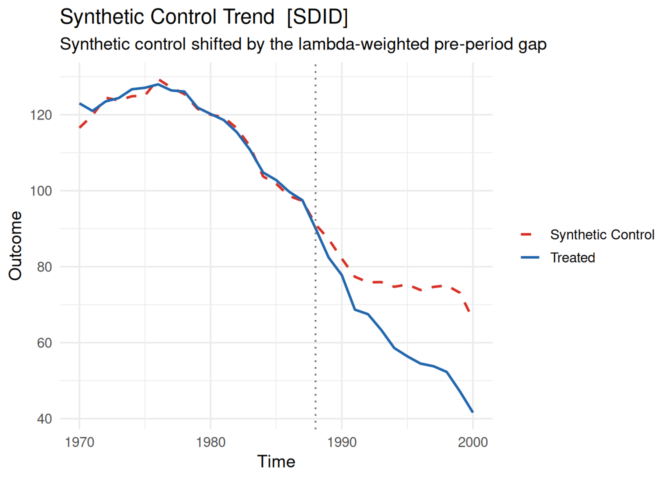

The synthetic California series is vertically shifted so that the pre-treatment time-weighted baseline matches California, making the post-1988 divergence immediately interpretable as the causal effect.

plot(core_sdid, type = "trend", align = FALSE)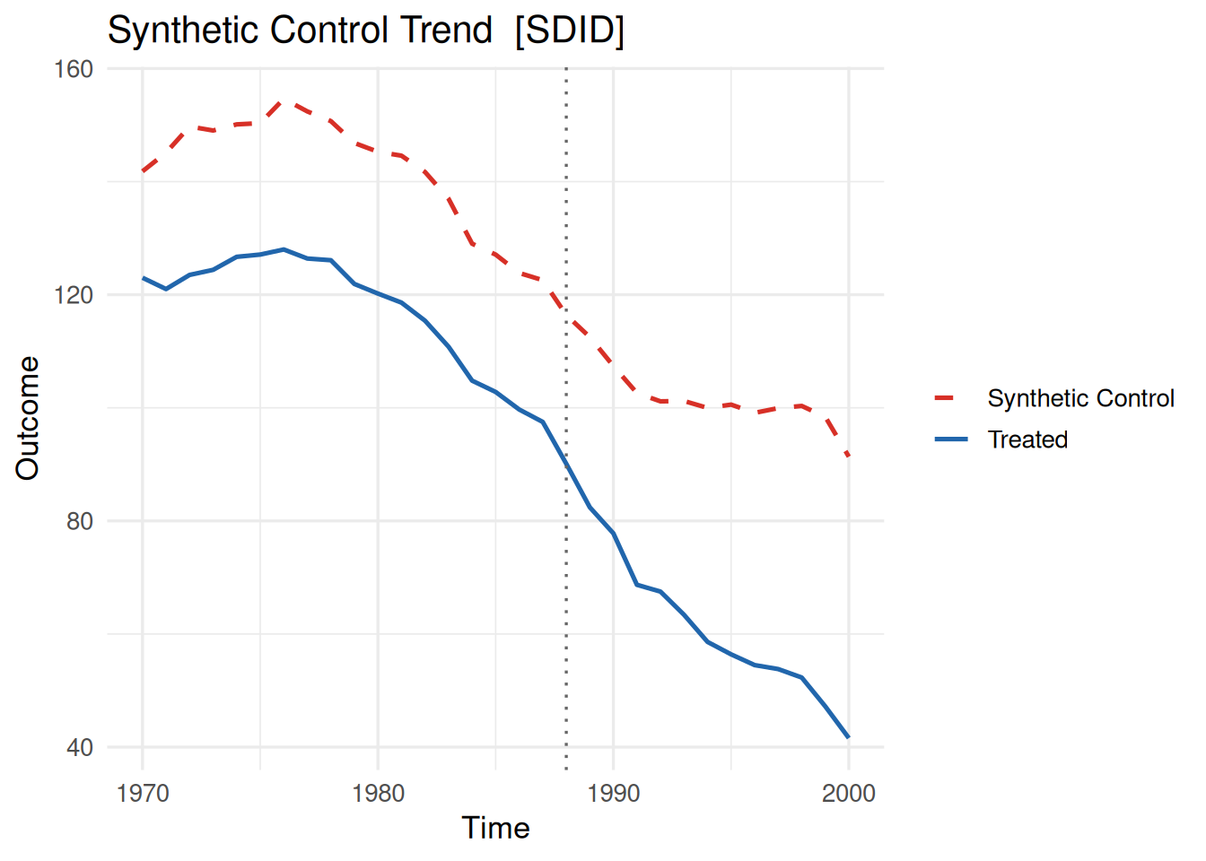

The raw plot illustrates the actual unadjusted levels of the synthetic composite compared to California, highlighting the presence of a baseline level difference that SDID effectively absorbs.

Gap Plot

The gap plot (type = "gap") plots the estimated treatment effect over time:

plot(core_sdid, type = "gap", align = TRUE)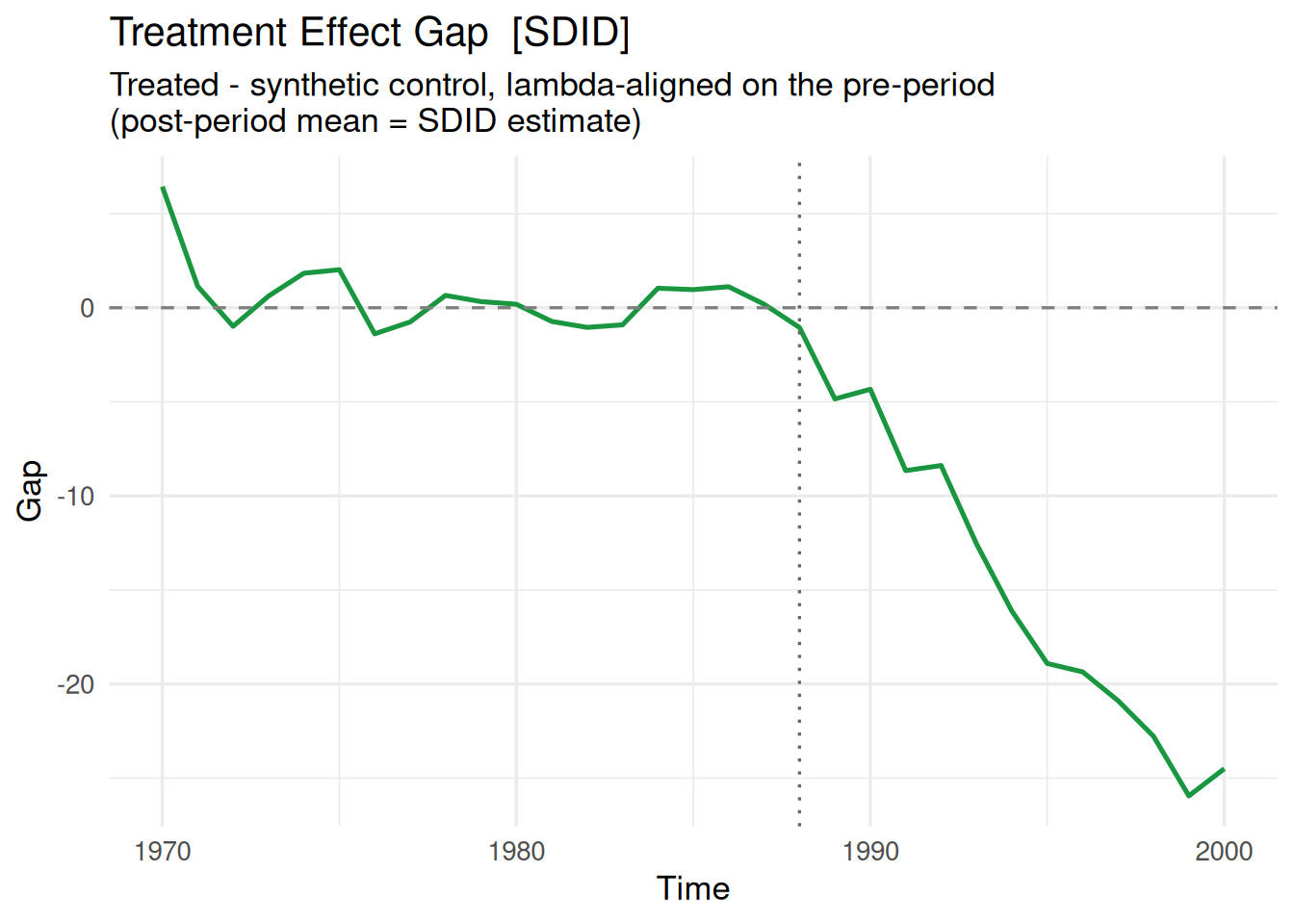

With align = TRUE, the pre-treatment gap fluctuates closely around zero, and the post-treatment line confirms the steady decrease in cigarette sales following the policy adoption.

Inspecting Unit and Time Weights

A key feature of SDID is that it solves for both unit weights ($\hat\omega_i$) and pre-treatment time weights ($\hat\lambda_t$). Calling plot(..., type = "weights") on an SDID object generates a two-panel chart displaying both weight vectors:

plot(core_sdid, type = "weights")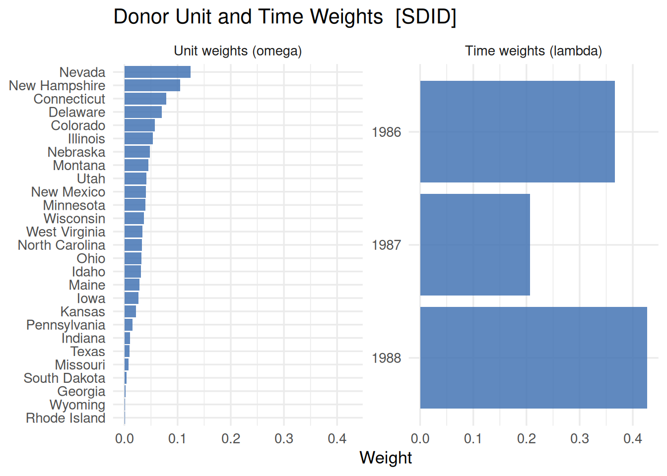

The top panel illustrates which donor states carry positive weight in constructing the synthetic counterfactual (e.g., Utah, Montana, Nevada). The bottom panel displays the time weights $\hat\lambda_t$, showing how recent pre-treatment years (such as 1987–1988) are prioritized to best match the trajectory leading up to the intervention.

Overlaying Donor Trajectories (`show_donors`)

To assess whether the synthetic control is interpolating plausibly among donor units, you can pass show_donors = N to draw the raw trajectories of the top $N$ donor states as thin background lines:

plot(core_sdid, type = "trend", align = TRUE, show_donors = 5)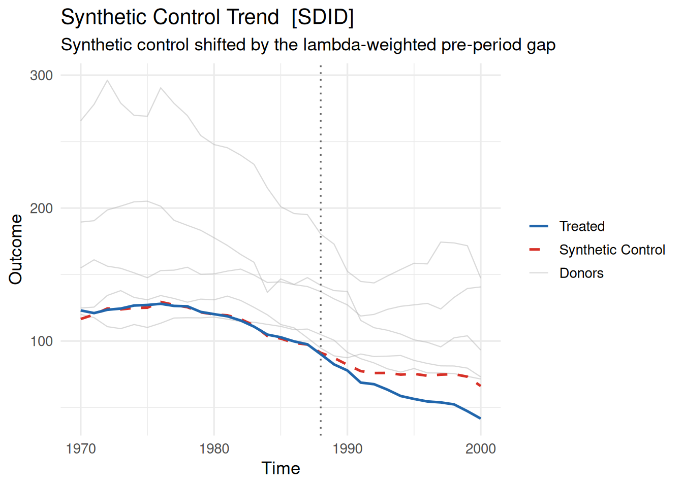

Customizing Plots with ggplot2

Because all coresynth plots are standard ggplot2 objects, you can easily customize styling, labels, colors, and line types using native ggplot2 grammar. For details on all arguments supported in plot(), see ?plot.coresynth.

plot(
  core_sdid,
  type = "trend",
  align = TRUE,
  colors = c(treated = "darkblue", synthetic = "firebrick"),
  labels = c(treated = "California (Observed)", synthetic = "SDID Counterfactual"),
  linetypes = c(treated = "solid", synthetic = "dashed"),
  vline = list(color = "black", linetype = "dotted"),
  vline_offset = -1
) +
  labs(
    title = "Cigarette Sales in California vs. Synthetic DID Counterfactual",
    subtitle = "Proposition 99 Tobacco Control Program (1988)",
    x = NULL,
    y = "Packs per Capita"
  ) +
  theme_minimal() +
  theme(legend.position = "bottom")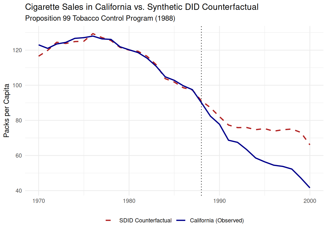

Statistical Inference with `sdid_inference()`

Quantifying statistical uncertainty is essential for credible causal evaluation. While SCM relied almost exclusively on permutation placebo tests (Abadie et al. 2010), SDID provides a framework with multiple inference methods (Arkhangelsky et al. 2021; Clarke et al. 2024).

In coresynth, statistical inference is unified under sdid_inference(). The function provides four primary inferential methods:

sdid_inference(
  fit,
  method      = c("placebo", "bootstrap", "jackknife", "jackknife_global"),
  n_boot      = 200L,
  level       = 0.95,
  alternative = c("two.sided", "greater", "less"),
  seed        = NULL
)

Choosing the Right Inference Method

The appropriate choice of inference method depends primarily on the design of your study and the questions being asked:

Single Treated Unit ($N_{\text{tr}} = 1$): When only one unit is treated (as in our California study), donor resampling alone cannot vary the treated unit’s idiosyncratic time-series shocks. In this setting, use method = "placebo" or Conformal Inference (conformal_inference()) to construct empirical benchmarks for hypothesis testing.
Assessing Donor Selection Uncertainty: The control bootstrap (method = "bootstrap") or jackknife (method = "jackknife") assesses sampling variability across the donor pool by resampling or dropping control units while holding the treated unit trajectories fixed.
Staggered Adoption ($N_{\text{tr}} \ge 2$ across cohorts): For roll-out designs where units adopt treatment at different times, use method = "jackknife_global" to account for cross-cohort covariance across the entire panel.
Distribution-Free Assumption: For finite-sample validity without parametric noise assumptions, use Conformal Inference via conformal_inference().

1. Placebo Permutation Inference (`method = "placebo"`)

For California Proposition 99, where $N_{\text{tr}} = 1$, we employ the in-space placebo permutation procedure (Algorithm 4 of Clarke et al. (2024) and Arkhangelsky et al. (2021)). Treatment is iteratively reassigned to each donor state to construct the empirical null distribution:

inf_placebo <- sdid_inference(core_sdid, method = "placebo")
inf_placebo

SDID Inference (placebo, alternative = two.sided)
  Estimate  : -15.6046 
  SE        : 9.3619 
  p-value   : 0.1026 
  CI        : [-33.9536, 2.7444]
  Controls  : 38

inf_placebo$p_value reports the two-sided permutation $p$-value. Additionally, sdid_inference() calculates the standard error as the standard deviation of the placebo distribution, alongside a normal-approximation 95% confidence interval (ci_lower and ci_upper).

Notice that because the placebo standard error assumes the treated unit’s noise variance is comparable to that of the donor units, it should be interpreted thoughtfully when donor pools are modest in size.

2. Unit Bootstrap (`method = "bootstrap"`)

In coresynth, method = "bootstrap" implements a donor bootstrap that draws $N_{\text{co}}$ control units with replacement from the donor pool while holding the treated series fixed, re-estimating unit weights $\hat\omega$ and time weights $\hat\lambda$ on each replicate. This evaluates standard errors and confidence intervals driven by donor-pool composition and weight uncertainty.

To illustrate how multi-unit inference operates in coresynth, let’s generate a synthetic panel with 4 treated units and 20 control units:

set.seed(42)
multi_panel <- expand.grid(unit = 1:24, year = 1990:2010)
multi_panel$treated <- as.integer(multi_panel$unit <= 4 & multi_panel$year >= 2002)
multi_panel$y <- multi_panel$unit * 1.5 + 0.8 * (multi_panel$year - 1990) +
  rnorm(nrow(multi_panel), sd = 0.5) - 2.5 * multi_panel$treated

fit_multi <- scm_fit(y ~ treated | unit + year, data = multi_panel, method = "sdid")

Now we execute the bootstrap with n_boot = 200:

inf_boot <- sdid_inference(fit_multi, method = "bootstrap", n_boot = 200, seed = 123)
inf_boot$se

[1] 0.1223251

inf_boot$p_value

[1] 1.537641e-105

c(inf_boot$ci_lower, inf_boot$ci_upper)

[1] -2.966984 -2.467841

3. Jackknife Variance Estimation (`method = "jackknife"`)

The jackknife drops one control unit at a time from the donor pool and recomputes the SDID estimator while holding the treated series fixed. Because it evaluates sensitivity to individual donor exclusions and avoids large quadratic programs, it runs almost instantaneously:

inf_jack <- sdid_inference(fit_multi, method = "jackknife")
inf_jack$se

[1] 0.09577276

inf_jack$p_value

[1] 6.531321e-171

For staggered adoption panels, method = "jackknife_global" drops each unit from the entire multi-cohort panel simultaneously, correctly preserving the covariance between cohorts.

4. Conformal Inference (`conformal_inference()`)

If you prefer hypothesis tests with exact finite-sample guarantees that avoid asymptotic approximations, coresynth provides Conformal Inference based on Chernozhukov et al. (2021). It constructs a moving-block permutation test under the null hypothesis of no treatment effect:

conf_res <- conformal_inference(core_sdid, level = 0.95)
conf_res$p_value

[1] 0.2903226

c(conf_res$ci_lower, conf_res$ci_upper)

[1] -27.129516  -4.079668

Dynamic Effects & Event Studies: `sdid_event_study()`

[!NOTE] sdid_event_study() is currently available only in the development version of coresynth (pak::pak("yo5uke/coresynth")).

Researchers often want to inspect dynamic treatment trajectories—confirming that pre-treatment coefficients are indistinguishable from zero (pre-trend check) while tracing out how effects unfold post-intervention.

coresynth provides the dedicated sdid_event_study() function for this purpose. It computes period-by-period treatment effects aligned on the $\hat\lambda$-weighted pre-treatment baseline. Crucially, the post-treatment average of the period-specific coefficients equals the aggregate SDID ATT (fit$estimate) exactly:

es_res <- sdid_event_study(
  fit_multi,
  n_boot = 100,
  seed = 42
)
es_res

=== SDID Event Study (unit bootstrap, 24 units) ===
  ATT Estimate : -2.669 
  ATT SE       : 0.1135 
  p-value      : < 1e-04 
  95% CI (norm): [-2.8914, -2.4466]
  95% CI (pct) : [-2.9837, -2.5178]
  Bootstrap    : 98 valid / 100 requested (2 discarded)

Period-by-period effects (lambda-aligned; post-period mean = ATT):
 time period estimate     se ci_norm_lower ci_norm_upper ci_pct_lower
 1990    pre   0.1855 0.2316       -0.2684        0.6395      -0.3647
 1991    pre   0.0835 0.3335       -0.5703        0.7372      -0.3977
 1992    pre  -0.0831 0.1697       -0.4157        0.2496      -0.3478
 1993    pre  -0.0381 0.2502       -0.5286        0.4523      -0.6192
 1994    pre  -0.1628 0.2465       -0.6460        0.3203      -0.6895
 1995    pre  -0.3078 0.1822       -0.6649        0.0493      -0.7070
 1996    pre   0.0934 0.1906       -0.2801        0.4670      -0.2366
 1997    pre   0.2562 0.1660       -0.0691        0.5815      -0.0919
 1998    pre  -0.0985 0.2764       -0.6403        0.4433      -0.7148
 1999    pre   0.0612 0.2430       -0.4150        0.5374      -0.2661
 2000    pre   0.3969 0.2307       -0.0552        0.8490      -0.0666
 2001    pre   0.1075 0.1336       -0.1543        0.3694      -0.1182
 2002   post  -2.7456 0.2947       -3.3232       -2.1680      -3.4195
 2003   post  -2.6668 0.1871       -3.0334       -2.3001      -3.0655
 2004   post  -2.9553 0.1733       -3.2949       -2.6156      -3.3258
 2005   post  -2.9730 0.1599       -3.2864       -2.6595      -3.2839
 2006   post  -2.5753 0.1357       -2.8413       -2.3094      -2.8663
 2007   post  -2.5470 0.4140       -3.3584       -1.7355      -3.4072
 2008   post  -2.5930 0.2884       -3.1583       -2.0276      -3.1925
 2009   post  -1.8374 0.3323       -2.4887       -1.1861      -2.4329
 2010   post  -3.1276 0.2292       -3.5768       -2.6784      -3.5492
 ci_pct_upper
       0.5440
       0.8012
       0.2906
       0.3748
       0.2228
      -0.0154
       0.5352
       0.5942
       0.3260
       0.6190
       0.7993
       0.4177
      -2.2548
      -2.3392
      -2.6547
      -2.7004
      -2.3832
      -1.7256
      -2.2045
      -1.1699
      -2.6808

Visualizing the Event Study

You can plot the event-study trajectory directly using the S3 plot() method:

plot(es_res)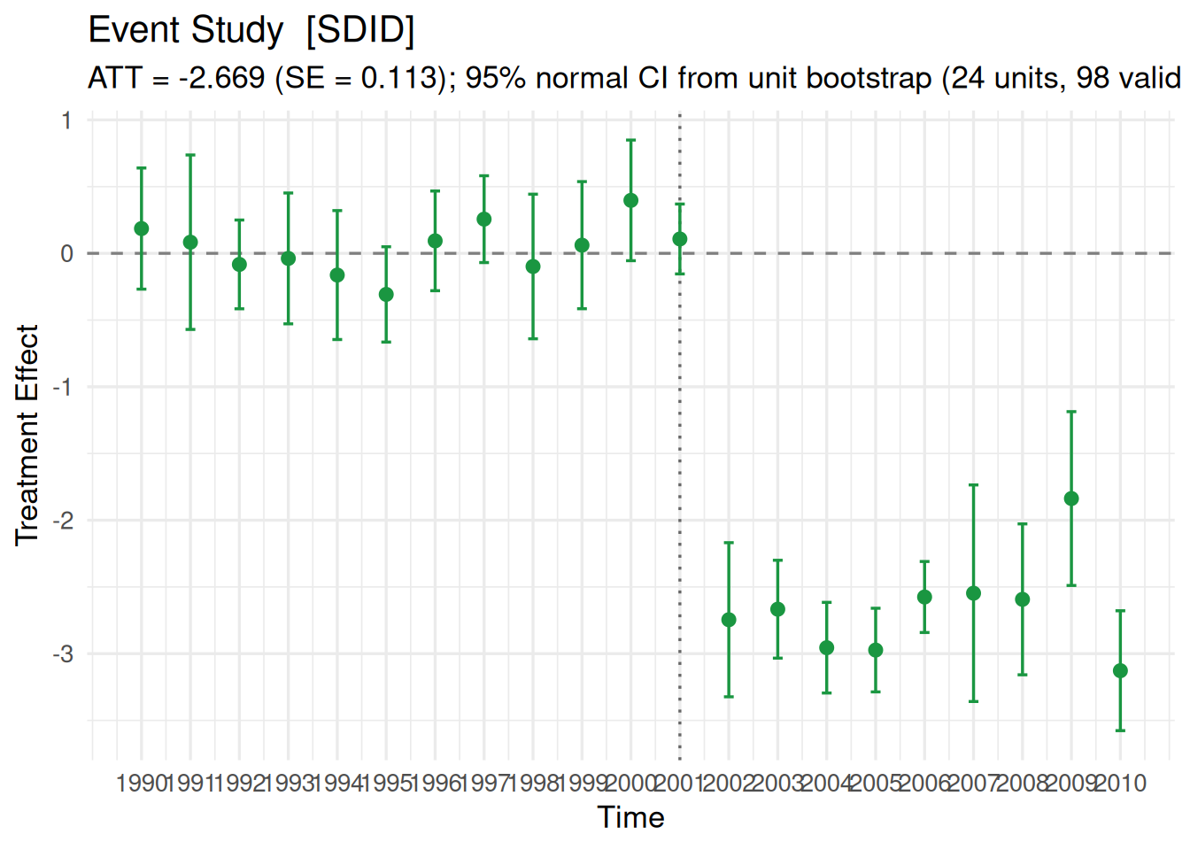

The resulting figure displays period-specific point estimates accompanied by confidence interval bands. The pre-treatment periods center closely around zero, validating the pre-trend fit, while the post-treatment drop vividly illustrates the causal effect over time.

Cluster Bootstrap Support

If units belong to geographical clusters (such as districts within states or prefectures), you can pass cluster = "cluster_var" and data = panel_df to sdid_event_study(). The function will perform block-cluster resampling of entire clusters with replacement, ensuring valid inference even in the presence of arbitrary intra-cluster correlation.

Advanced Topics

Time-Varying Covariates

SDID supports adjusting for time-varying confounders via the covariates argument. Following Clarke et al. (2024) and Arkhangelsky et al. (2021), covariates are residualized out of the outcome using two-way fixed effects before computing the unit and time weights:

# Example with time-varying covariates (e.g., retail price)
fit_cov <- scm_fit(
  cigsale ~ treated | state + year,
  data = smoking,
  method = "sdid",
  covariates = "retprice"
)
summary(fit_cov)

Staggered Adoption

When different units receive treatment at different points in time, coresynth automatically detects the staggered timing and applies the cohort aggregation framework of Clarke et al. (2024):

# Staggered adoption SDID fit
fit_stagg <- scm_fit(
  y ~ treated | unit + year,
  data = staggered_panel,
  method = "sdid",
  control_group = "never_treated" # Default in v1.0.0+
)
fit_stagg$cohort_estimates

In coresynth 1.0.0 and later, control_group = "never_treated" is the default, ensuring that only pure, never-treated units serve as donors for each adoption cohort to prevent contamination from future adopters.

Tidy Ecosystem Integration & JSON Export

To ensure smooth integration into reproducible research pipelines, coresynth fully supports {broom} tidying methods and structured JSON serialization:

Broom Integration: `tidy()` and `glance()`

broom::tidy(inf_placebo)

  term  estimate std.error statistic   p.value  conf.low conf.high  method
1  ATT -15.60459  9.361917 -1.666816 0.1025641 -33.95361  2.744429 placebo
  alternative n_controls staggered
1   two.sided         38     FALSE

broom::glance(inf_placebo)

   method n_controls staggered  estimate std.error   p.value  conf.low
1 placebo         38     FALSE -15.60459  9.361917 0.1025641 -33.95361
  conf.high alternative n_boot_valid
1  2.744429   two.sided           NA

Extracting Tidy Data via `plot_data()`

If you wish to create fully custom visualizations in ggplot2 or export tabular summaries, plot_data() provides raw data frames:

# Extract aligned trend data
plot_data(core_sdid, type = "trend", align = TRUE) |> head()

  time value  series
1 1970 123.0 Treated
2 1971 121.0 Treated
3 1972 123.5 Treated
4 1973 124.4 Treated
5 1974 126.7 Treated
6 1975 127.1 Treated

# Extract unit and time weights
plot_data(core_sdid, type = "weights") |> head()

         unit      weight panel
1     Alabama 0.000000000 omega
2    Arkansas 0.000000000 omega
3    Colorado 0.057429525 omega
4 Connecticut 0.078401014 omega
5    Delaware 0.070446947 omega
6     Georgia 0.001986351 omega

Exporting Results to JSON

For cross-language pipelines (e.g., Python, dashboards) and archiving, use export_json():

export_json(core_sdid, file = "sdid_results.json", inference = inf_placebo)

Summary & Feedback

Synthetic Difference-in-Differences is an estimator that addresses the weaknesses of both standard DID and classical SCM. With {coresynth}, running SDID is as simple as writing a standard regression formula, backed by fast C++ optimization, along with versatile tools for inference and visualization.

I hope coresynth helps accelerate your causal inference workflow.

If you have any questions, encounter bugs, or would like to request new features, please feel free to open an issue on the GitHub Repository or reach out on X (@5uke_y)!

References

Abadie, Alberto, Alexis Diamond, and Jens Hainmueller. 2010. "Synthetic Control Methods for Comparative Case Studies: Estimating the Effect of California’s Tobacco Control Program". Journal of the American Statistical Association 105 (490): 493–505. https://doi.org/10.1198/jasa.2009.ap08746.

Arkhangelsky, Dmitry, Susan Athey, David A. Hirshberg, Guido W. Imbens, and Stefan Wager. 2021. "Synthetic Difference-in-Differences". American Economic Review 111 (12): 4088–118. https://doi.org/10.1257/aer.20190159.

Chernozhukov, Victor, Kaspar Wüthrich, and Yinchu Zhu. 2021. "An Exact and Robust Conformal Inference Method for Counterfactual and Synthetic Controls". Journal of the American Statistical Association 116 (536): 1849–64. https://doi.org/10.1080/01621459.2021.1920957.

Clarke, Damian, Daniel Pailañir, Susan Athey, and Guido Imbens. 2024. "On Synthetic Difference-in-Differences and Related Estimation Methods in Stata". The Stata Journal 24 (4): 557–98. https://doi.org/10.1177/1536867X241297914.