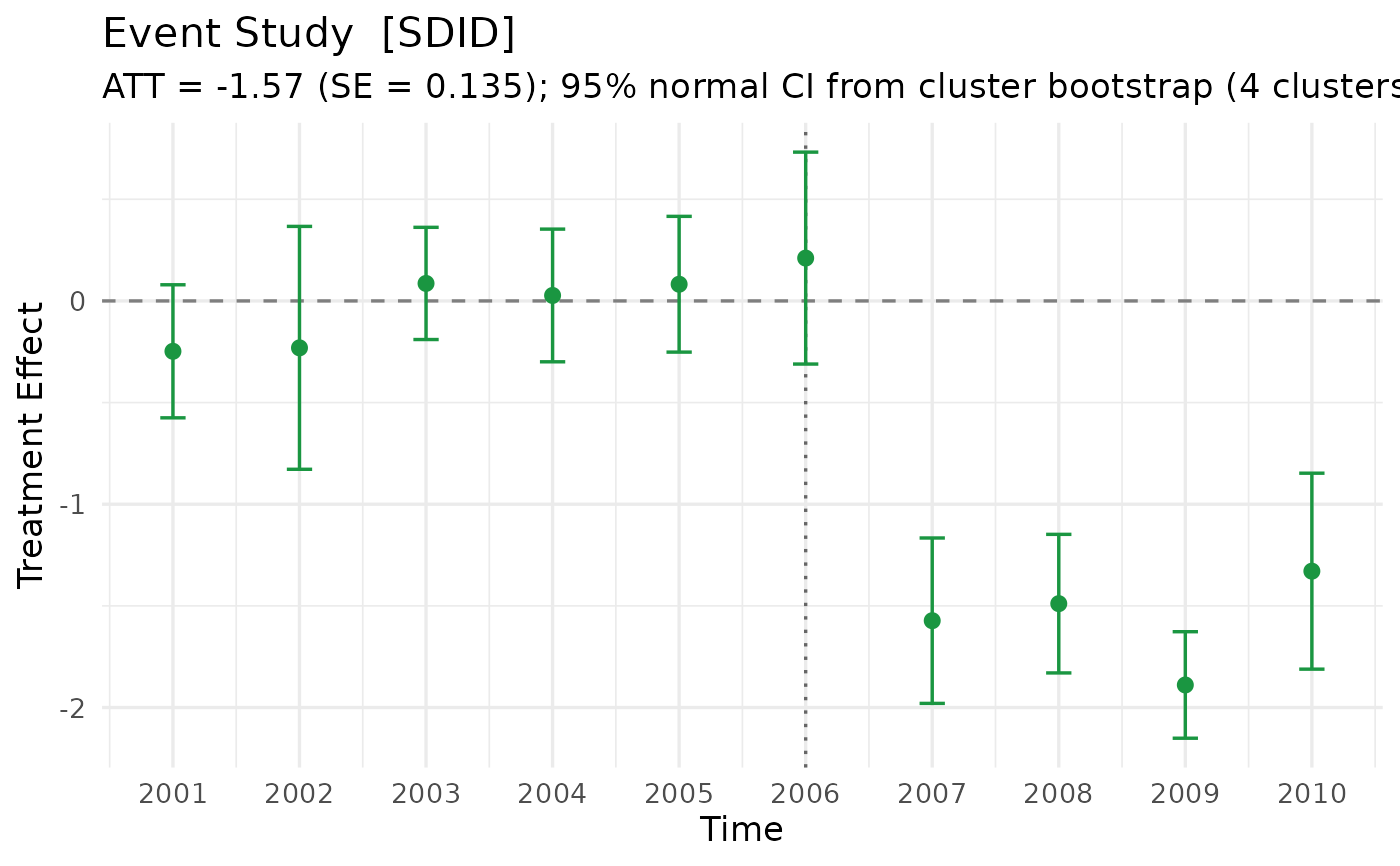
Event Study with Cluster or Unit Bootstrap for SDID

Computes period-by-period treatment effects (event-study series) for a sharp Synthetic Difference-in-Differences fit, aligned on the $\hat\lambda$-weighted pre-treatment gap so that the post-treatment mean of the period effects equals the SDID ATT (fit$estimate) exactly, together with bootstrap standard errors and confidence intervals (both normal approximation and percentile) for every period and for the overall ATT from the same bootstrap draws.

Usage

sdid_event_study(
  fit,
  cluster = NULL,
  data = NULL,
  n_boot = 200L,
  level = 0.95,
  ci_type = c("normal", "percentile"),
  seed = NULL
)

Arguments

fit

A sharp coresynth object fitted with method = "sdid". Staggered fits are not supported and raise an error.

cluster

Cluster specification for block/cluster bootstrap resampling (e.g. prefecture or state):

NULL (default): resample individual units (both treated and control) with replacement.
A single character string naming a column in data (or a one-sided formula ~ col), in which case data must also be supplied.
A named vector whose names are unit IDs matching the units in fit and whose values give each unit's cluster ID.

Unnamed positional vectors are rejected to prevent silent misalignment between row/column order and unit IDs.

data

Optional data.frame containing the unit identifier column and the cluster column when cluster is given as a column name.

n_boot

Integer number of bootstrap replications (default 200L). Set n_boot = 0L (or NULL) to skip the bootstrap and return point estimates only.

level

Confidence level for the intervals (default 0.95).

ci_type

Which confidence interval type ("normal" or "percentile") to populate conf.low and conf.high with in tidy(), glance(), and plot() by default. Both normal-approximation (ci_norm_lower, ci_norm_upper) and percentile (ci_pct_lower, ci_pct_upper) intervals are always computed and stored.

seed

Optional integer seed for reproducible bootstrap resampling.

Value

An object of class "sdid_event_study" (a named list) containing:

terms: A data.frame with one row per period (time, event_time, period ("pre" / "post"), estimate, se, ci_norm_lower, ci_norm_upper, ci_pct_lower, ci_pct_upper, conf.low, conf.high). mean(terms$estimate[terms$period == "post"]) equals estimate (ATT).
estimate: Overall SDID ATT (fit$estimate).
se: Bootstrap standard error of the ATT (sd(boot_att)).
p_value: Two-sided normal-approximation p-value for the ATT.
ci_norm_lower, ci_norm_upper: Normal-approximation CI for the ATT.
ci_pct_lower, ci_pct_upper: Percentile CI for the ATT.
ci_lower, ci_upper: ATT CI bounds matching ci_type.
ci_type: Resolved default CI type ("normal" or "percentile").
level: Confidence level.
n_boot: Requested number of bootstrap draws.
n_boot_valid: Number of valid bootstrap draws completed.
n_boot_dropped: Number of draws discarded (empty treated/control group or solver failure).
clustered: Logical; TRUE when cluster was supplied.
n_clusters: Number of unique clusters (or total units when unclustered).
n_treated: Number of treated units in fit.
n_controls: Number of control units in fit.
times: Time index vector (fit$times).
T_pre: Number of pre-treatment periods (fit$T_pre).
boot_gaps: Numeric matrix of dimension n_boot_valid x T holding the aligned period-by-period gap series for each valid bootstrap draw (colnames are as.character(times)), or NULL when n_boot == 0.
boot_att: Numeric vector of length n_boot_valid holding the ATT for each valid draw (identical to rowMeans(boot_gaps[, (T_pre + 1):T])), or NULL when n_boot == 0.

Details

Resampling scheme: As in sdid_inference() with method = "bootstrap" (Arkhangelsky et al. 2021, Algorithm 2), sdid_event_study() resamples both treated and control units with replacement – here at the cluster level when cluster is supplied, or at the unit level when cluster = NULL – and reports period-by-period effects as well as the ATT. Duplicated units in a bootstrap draw enter as distinct unit columns (equivalent to assigning fresh unit IDs per draw), and $\hat\sigma^2$, $\zeta^2$ (unless user-fixed in scm_fit()), unit weights $\hat\omega$, and time weights $\hat\lambda$ are all re-estimated on each draw. Draws in which either the resampled treated group or the resampled control group has zero units (or fewer than two control units) are discarded; the counts of valid and discarded draws are reported in n_boot_valid and n_boot_dropped.

Pre-treatment period coefficients are returned and plotted for visual inspection of pre-trends only; no joint Wald test is performed because the pre-treatment gaps are constrained by the $\hat\omega$ and $\hat\lambda$ weights and their covariance matrix can be singular.

Examples

set.seed(1)
panel <- expand.grid(unit = 1:12, year = 2001:2010)
panel$pref <- paste0("pref_", (panel$unit - 1) %% 4 + 1)
panel$d <- as.integer(panel$unit <= 3 & panel$year >= 2007)
panel$y <- panel$unit + 0.5 * (panel$year - 2000) +
  rnorm(nrow(panel), sd = 0.3) - 1.5 * panel$d

fit <- scm_fit(y ~ d | unit + year, data = panel, method = "sdid")
es  <- sdid_event_study(fit, cluster = "pref", data = panel,
                        n_boot = 50, seed = 42)
es
#> === SDID Event Study (cluster bootstrap, 4 clusters) ===
#>   ATT Estimate : -1.57 
#>   ATT SE       : 0.1353 
#>   p-value      : < 1e-04 
#>   95% CI (norm): [-1.8353, -1.3048]
#>   95% CI (pct) : [-1.9090, -1.3526]
#>   Bootstrap    : 50 valid / 50 requested (0 discarded)
#> 
#> Period-by-period effects (lambda-aligned; post-period mean = ATT):
#>  time period estimate     se ci_norm_lower ci_norm_upper ci_pct_lower
#>  2001    pre  -0.2478 0.1670       -0.5750        0.0794      -0.7314
#>  2002    pre  -0.2308 0.3048       -0.8282        0.3665      -0.6683
#>  2003    pre   0.0860 0.1408       -0.1899        0.3619      -0.1722
#>  2004    pre   0.0268 0.1665       -0.2995        0.3531      -0.2358
#>  2005    pre   0.0820 0.1703       -0.2518        0.4159      -0.3415
#>  2006    pre   0.2106 0.2659       -0.3106        0.7318      -0.1574
#>  2007   post  -1.5728 0.2075       -1.9796       -1.1661      -1.8904
#>  2008   post  -1.4890 0.1739       -1.8298       -1.1482      -1.9003
#>  2009   post  -1.8890 0.1337       -2.1509       -1.6270      -2.0845
#>  2010   post  -1.3293 0.2459       -1.8112       -0.8474      -1.9274
#>  ci_pct_upper
#>        0.0137
#>        0.3890
#>        0.3809
#>        0.3698
#>        0.3422
#>        0.7224
#>       -1.0800
#>       -1.1575
#>       -1.5637
#>       -0.8558
broom::tidy(es)
#>    time event_time period    estimate std.error   conf.low  conf.high
#> 1  2001         -6    pre -0.24782666 0.1669505 -0.5750436  0.0793903
#> 2  2002         -5    pre -0.23082454 0.3047693 -0.8281615  0.3665124
#> 3  2003         -4    pre  0.08600379 0.1407890 -0.1899376  0.3619452
#> 4  2004         -3    pre  0.02683772 0.1664804 -0.2994578  0.3531333
#> 5  2005         -2    pre  0.08204119 0.1703369 -0.2518129  0.4158953
#> 6  2006         -1    pre  0.21062669 0.2659272 -0.3105810  0.7318344
#> 7  2007          0   post -1.57284709 0.2075459 -1.9796296 -1.1660646
#> 8  2008          1   post -1.48899791 0.1738763 -1.8297892 -1.1482066
#> 9  2009          2   post -1.88898248 0.1336520 -2.1509356 -1.6270294
#> 10 2010          3   post -1.32930106 0.2458848 -1.8112264 -0.8473758
#>    ci_norm_lower ci_norm_upper ci_pct_lower ci_pct_upper
#> 1     -0.5750436     0.0793903   -0.7313559   0.01366954
#> 2     -0.8281615     0.3665124   -0.6682882   0.38901647
#> 3     -0.1899376     0.3619452   -0.1722406   0.38091707
#> 4     -0.2994578     0.3531333   -0.2357820   0.36984832
#> 5     -0.2518129     0.4158953   -0.3415019   0.34220943
#> 6     -0.3105810     0.7318344   -0.1574213   0.72242913
#> 7     -1.9796296    -1.1660646   -1.8903653  -1.08003971
#> 8     -1.8297892    -1.1482066   -1.9003357  -1.15754682
#> 9     -2.1509356    -1.6270294   -2.0844596  -1.56372942
#> 10    -1.8112264    -0.8473758   -1.9273740  -0.85579826
# \donttest{
plot(es)

# }

Usage

Arguments

Value

Details

See also

Examples