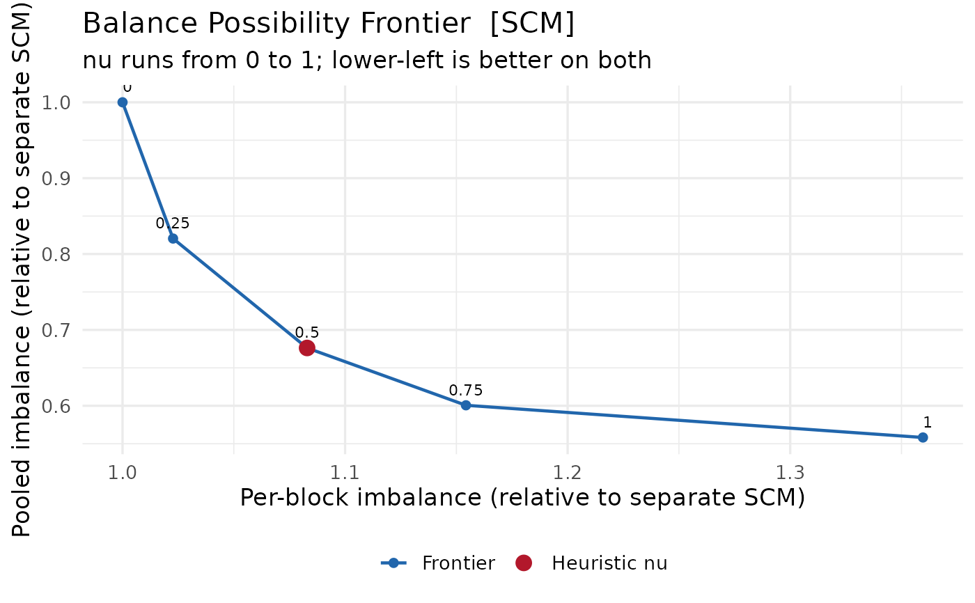
Draws the trade-off traced by scm_balance_frontier(): the imbalance of the
treated average, which the aggregate ATT rests on, against the root mean
square of the per-block imbalances, which the block-level effects rest on.
Separate SCM sits at one end of the curve and fully pooled SCM at the other,
with the heuristic the fit used marked along it.
Usage
# S3 method for class 'scm_frontier'
plot(x, relative = TRUE, label_nu = TRUE, colors = NULL, ...)
Arguments
- x
An
scm_frontierobject fromscm_balance_frontier().- relative
Plot the imbalances normalised by the separate solution (default), which puts both axes on comparable scales, rather than in the outcome's own units.
- label_nu
Annotate the drawn points with their
nu.- colors
Optional named overrides for the
"frontier"line and the"heuristic"marker.- ...
Ignored.
Details
The curve is normally strongly convex, which is the point of looking at it:
a small move away from either end usually buys a large reduction in the
other imbalance for very little, so the interesting values of nu are the
ones near the bend.
Examples
set.seed(1)
panel <- expand.grid(unit = 1:15, year = 1:20)
adopt <- c(`1` = 12, `2` = 15, `3` = 17)
panel$treated <- as.integer(!is.na(adopt[as.character(panel$unit)]) &
  panel$year >= adopt[as.character(panel$unit)])
panel$treated[is.na(panel$treated)] <- 0L
panel$gdp <- panel$unit + 0.4 * panel$year +
  rnorm(nrow(panel)) + 2 * panel$treated
fit <- scm_fit(gdp ~ treated | unit + year, data = panel, method = "scm")
plot(scm_balance_frontier(fit, nu_grid = c(0, 0.25, 0.5, 0.75, 1)))