fixes

Overview

fixes is an R package for difference-in-differences estimation in panel data. It covers the three stages of a modern DiD workflow:

Stage	Function	What it does
1. Event study	event_study()	Dynamic treatment effects by relative time (6 estimators)
2. ATT aggregation	att()	Aggregated ATT — overall, by cohort, by calendar time
3. Basic DiD	did()	Single-coefficient TWFE DiD with modelsummary support
4. Sensitivity	honest_sensitivity()	Robust inference under violations of parallel trends (Rambachan & Roth 2023)
Visualisation	plot()	Every result has a base plot() method (ggplot2); plot(x, interactive = TRUE) gives a plotly chart, plot(att_gt(x)) the ATT(g,t) heatmap/facets

Estimation runs on the package’s internal C++ fixed-effects OLS engine — fixest is an optional (suggested) dependency, not a requirement.

Upgrading from < 1.0.0? The verb-style API (run_es(), calc_att(), run_did(), plot_es(), …) still works and returns identical results, but is deprecated. See NEWS.md for the old-to-new mapping.

Estimators (selected via the estimator argument in event_study() and att()):

estimator	Reference	Best for
"twfe"	Classic TWFE	Universal treatment timing
"cs"	Callaway & Sant’Anna (2021)	Staggered adoption
"sa"	Sun & Abraham (2021)	Staggered adoption
"bjs"	Borusyak, Jaravel & Spiess (2024)	Staggered adoption
"twm"	Wooldridge (2025)	Staggered adoption; optional cohort trends
"flex"	Deb, Norton, Wooldridge & Zabel (2024)	Repeated cross-section data

Installation

# From CRAN
install.packages("fixes")

# Development version
pak::pak("yo5uke/fixes")

Quick start

library(fixes)

---

Basic DiD — did()

For a simple two-way FE DiD with a single treatment coefficient, use did(). Output is fully compatible with modelsummary::modelsummary() and tinytable::tt().

There are two equivalent ways to specify the treatment:

# Option A: supply a pre-built D_it indicator
df$D <- as.integer(df$treated & df$year >= 2006)
res <- did(df, outcome = y, treatment = D, fe = ~ id + year)

# Option B: let did() construct D_it from group indicator + timing
res <- did(df, outcome = y, treatment = treated,
               time = year, timing = 2006,
               fe = ~ id + year)

Both options produce a did_result object:

df <- fixest::base_did

# Build a universal-timing DiD dataset
df$D <- as.integer(df$treat == 1 & df$period >= 5)

res <- did(
  data    = df,
  outcome = y,
  treatment = D,
  fe      = ~ id + period,
  cluster = ~ id
)

print(res)

## DiD Estimation  [TWFE]
## N = 1080 obs | 330 treated obs
## FE: id + period 
## VCOV: cluster | Cluster: id 
## 
##   term estimate std.error statistic  p.value
## 1    D      4.5     0.544      8.27 3.94e-13

did() integrates with the broom and modelsummary ecosystems:

broom::tidy(res)          # all coefficients (treatment + any covariates)
broom::glance(res)        # nobs, within R², AIC, ...
modelsummary::modelsummary(res)   # regression table via tinytable

---

Event study — event_study()

All six estimators share the same interface.

Classic TWFE (single treatment date)

Use event_study() with a fixed event date. Here we use fixest::base_did, a balanced panel where all units are treated at period 5.

es <- event_study(
  data      = df,
  outcome   = y,
  treatment = treat,
  time      = period,
  timing    = 5,
  fe        = ~ id + period,
  cluster   = ~ id,
  baseline  = -1
)

print(es)

## Event Study Result (fixes)
##   N: 1080  | Units: NA  | Treated units: 1080  | Never-treated: NA 
##   FE: id + period
##   VCOV: cluster  | Cluster: id 
##   Estimator: twfe 
##   Method: classic  | lead_range: 4  lag_range: 5  baseline: -1

plot(es)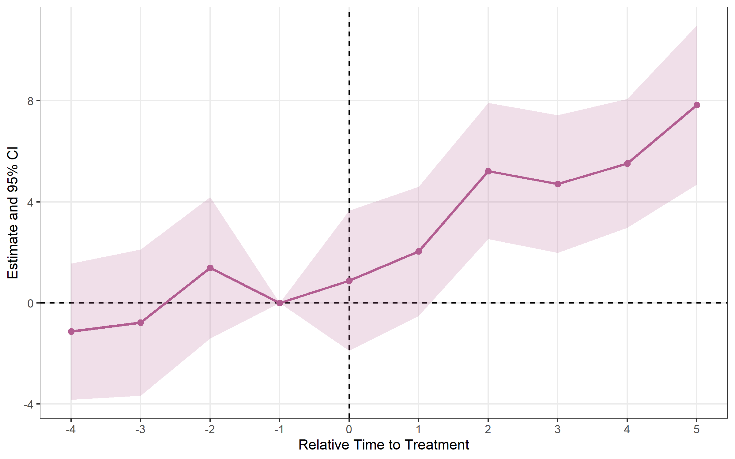

---

Staggered adoption

When units adopt treatment at different times, the classic TWFE estimator can be biased. fixes provides modern alternatives.

Setup: fixest::base_stagg — never-treated units have NA timing.

df_stagg <- fixest::base_stagg
df_stagg$timing <- df_stagg$year_treated
df_stagg$timing[df_stagg$year_treated == 10000] <- NA

Callaway & Sant’Anna (2021) — estimator = "cs"

cs <- event_study(
  data          = df_stagg,
  outcome       = y,
  time          = year,
  timing        = timing,
  unit          = id,
  staggered     = TRUE,
  estimator     = "cs",
  control_group = "nevertreated"
)

print(cs)

## Event Study Result (fixes)
##   N: 950  | Units: 95  | Treated units: 45  | Never-treated: 50 
##   FE: 
##   VCOV: analytic  | Cluster: - 
##   Estimator: cs 
##   Method: classic  | lead_range: 9  lag_range: 8  baseline: -1

plot(cs)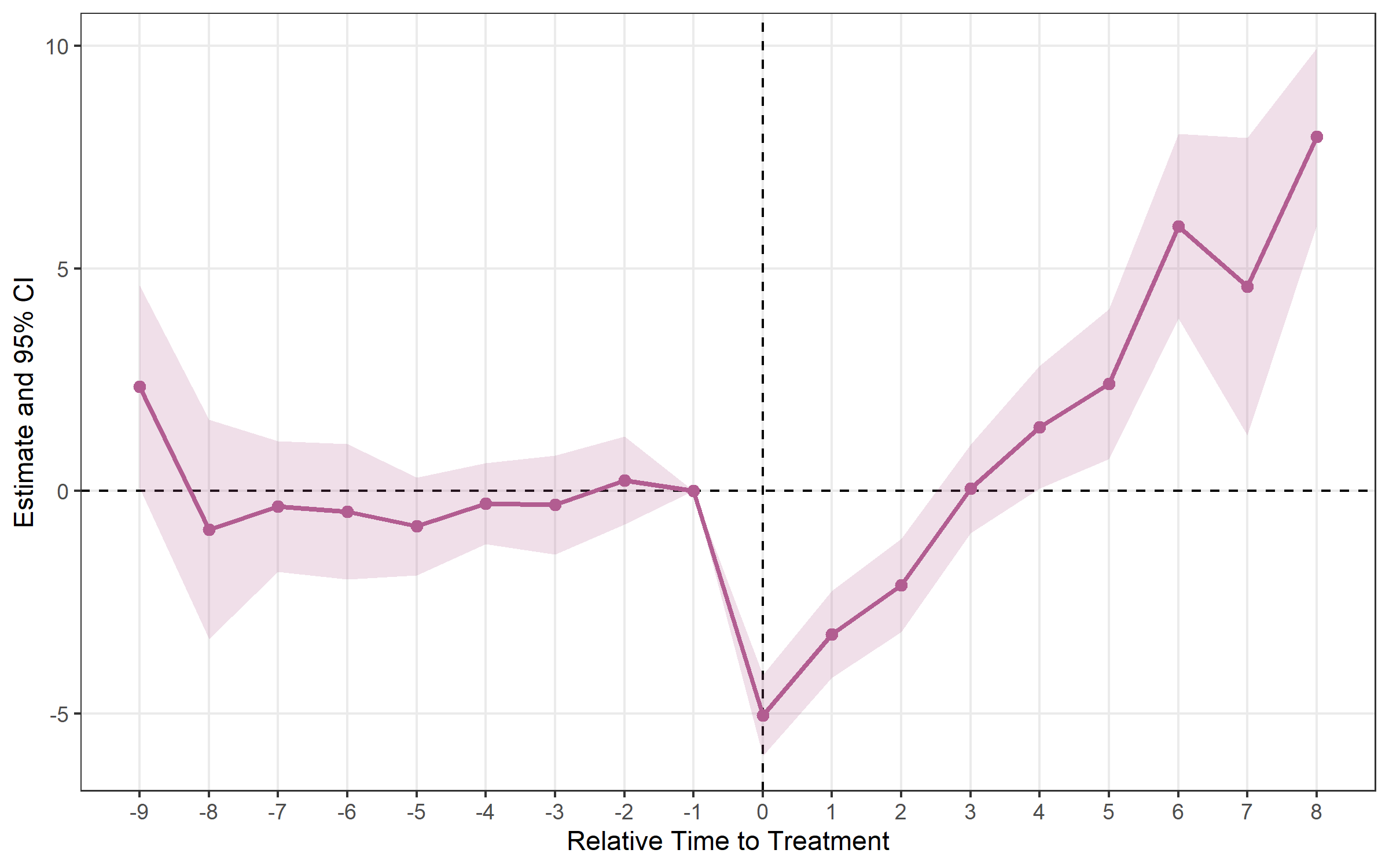

Visualise the full ATT(g,t) matrix

plot(att_gt(cs), type = "heatmap")

plot(att_gt(cs), type = "facet")

---

Sun & Abraham (2021) — estimator = "sa"

sa <- event_study(
  data      = df_stagg,
  outcome   = y,
  treatment = treated,
  time      = year,
  timing    = timing,
  unit      = id,
  fe        = ~ id + year,
  staggered = TRUE,
  estimator = "sa",
  cluster   = ~ id
)

print(sa)

## Event Study Result (fixes)
##   N: 950  | Units: 95  | Treated units: 45  | Never-treated: 50 
##   FE: id + year
##   VCOV: HC1  | Cluster: id 
##   Estimator: sa 
##   Method: classic  | lead_range: 9  lag_range: 8  baseline: -1

plot(sa)

---

Borusyak, Jaravel & Spiess (2024) — estimator = "bjs"

bjs <- event_study(
  data      = df_stagg,
  outcome   = y,
  time      = year,
  timing    = timing,
  unit      = id,
  staggered = TRUE,
  estimator = "bjs"
)

print(bjs)

## Event Study Result (fixes)
##   N: 950  | Units: 95  | Treated units: 45  | Never-treated: 50 
##   FE: id + year
##   VCOV: bjs_conservative  | Cluster: - 
##   Estimator: bjs 
##   Method: classic  | lead_range: 1  lag_range: 8  baseline: -1

plot(bjs)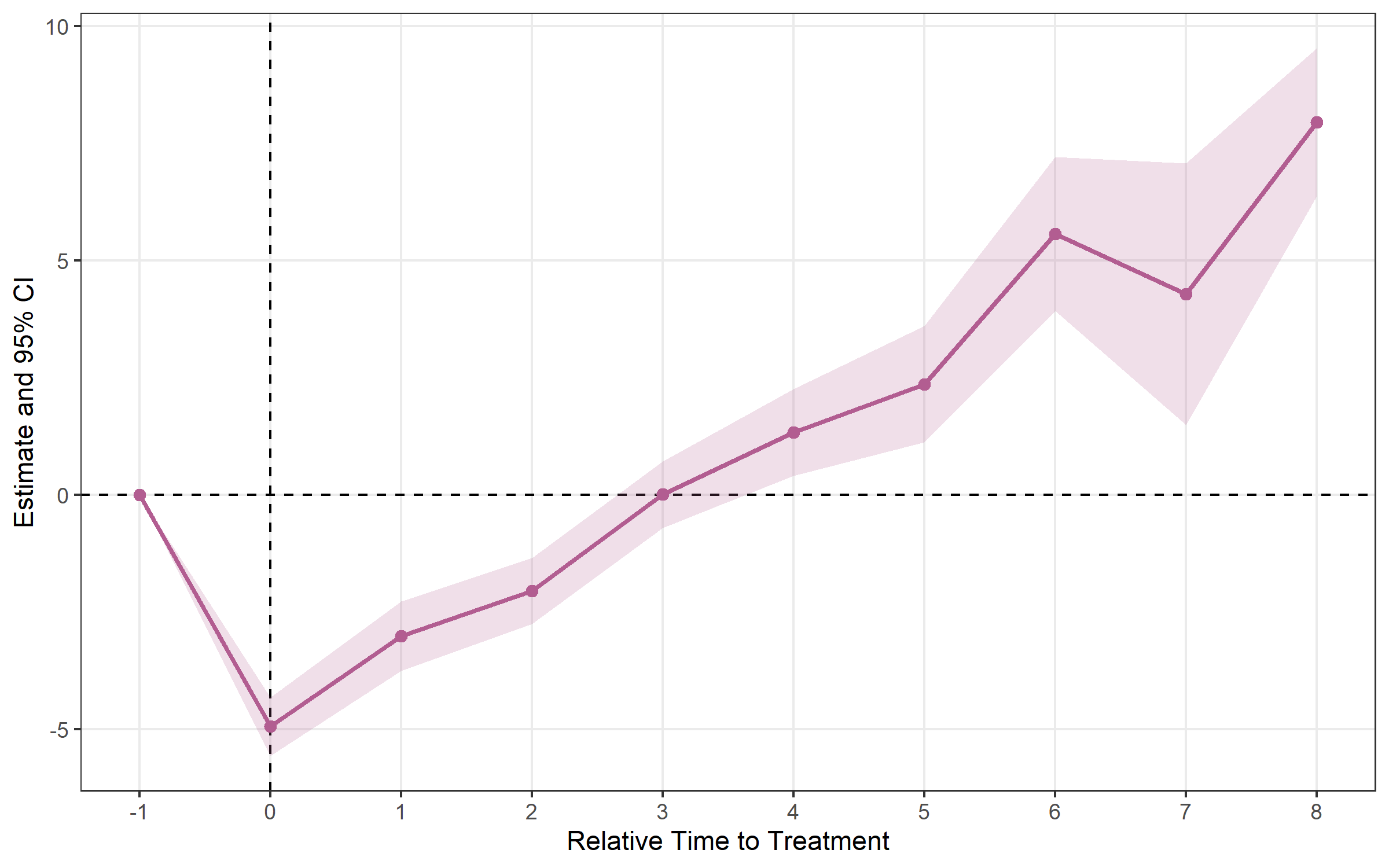

---

Wooldridge (2025) Two-Way Mundlak — estimator = "twm"

Algebraically equivalent to Sun-Abraham in the base case. trends = TRUE adds cohort-specific linear trend regressors to absorb differential pre-trends (output shows relative_time ≥ 0 only).

twm <- event_study(
  data      = df_stagg,
  outcome   = y,
  time      = year,
  timing    = timing,
  unit      = id,
  fe        = ~ id + year,
  staggered = TRUE,
  estimator = "twm"
)

print(twm)

## Event Study Result (fixes)
##   N: 950  | Units: 95  | Treated units: 45  | Never-treated: 50 
##   FE: id + year
##   VCOV: HC1  | Cluster: - 
##   Estimator: twm 
##   Method: classic  | lead_range: 9  lag_range: 8  baseline: -1

plot(twm)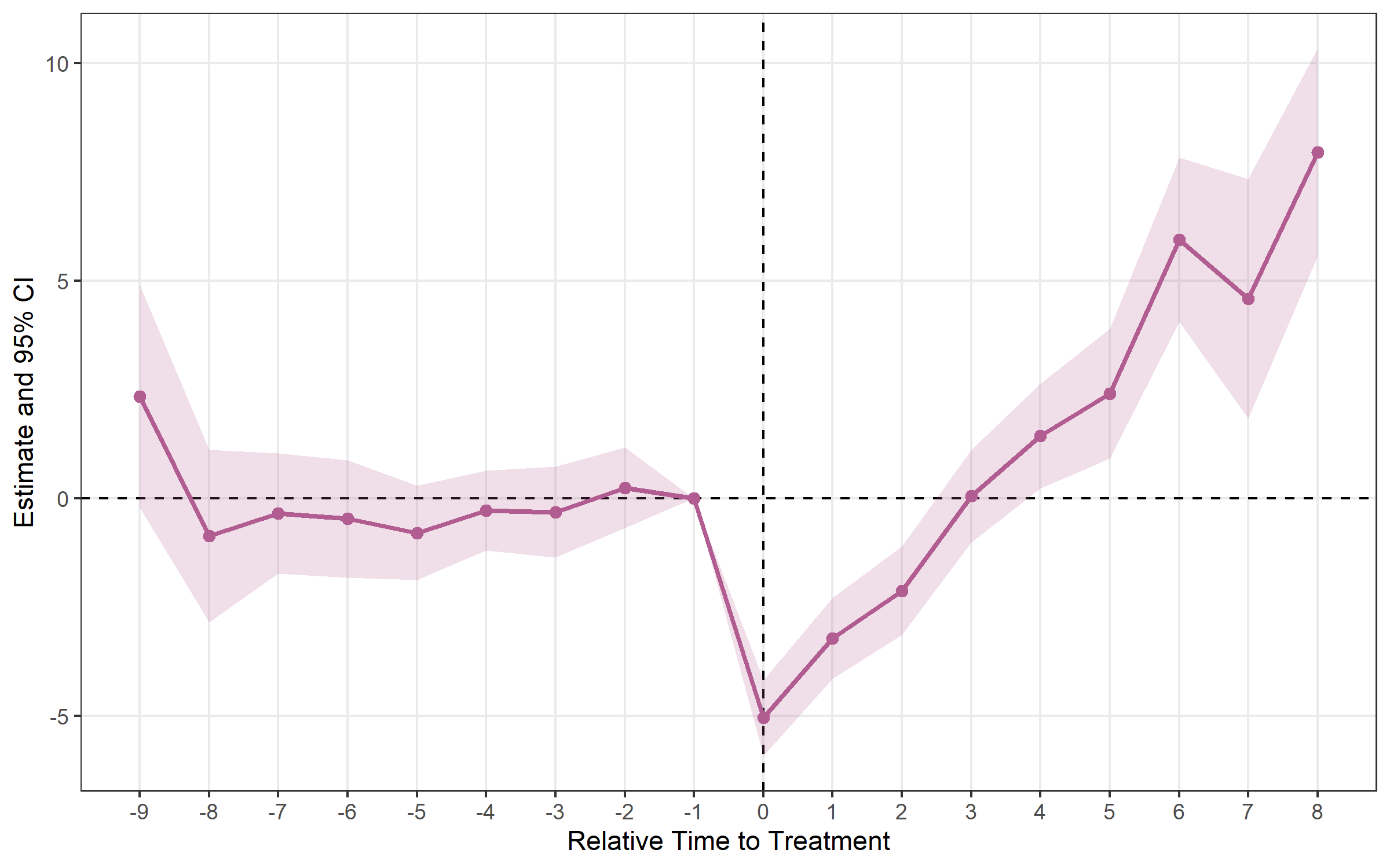

---

Deb, Norton, Wooldridge & Zabel (2024) FLEX — estimator = "flex"

Designed for repeated cross-section data (different individuals each period). Requires a group argument identifying the treatment group each observation belongs to.

flex <- event_study(
  data      = df_rcs,
  outcome   = y,
  time      = year,
  timing    = timing,
  group     = group_id,
  staggered = TRUE,
  estimator = "flex"
)

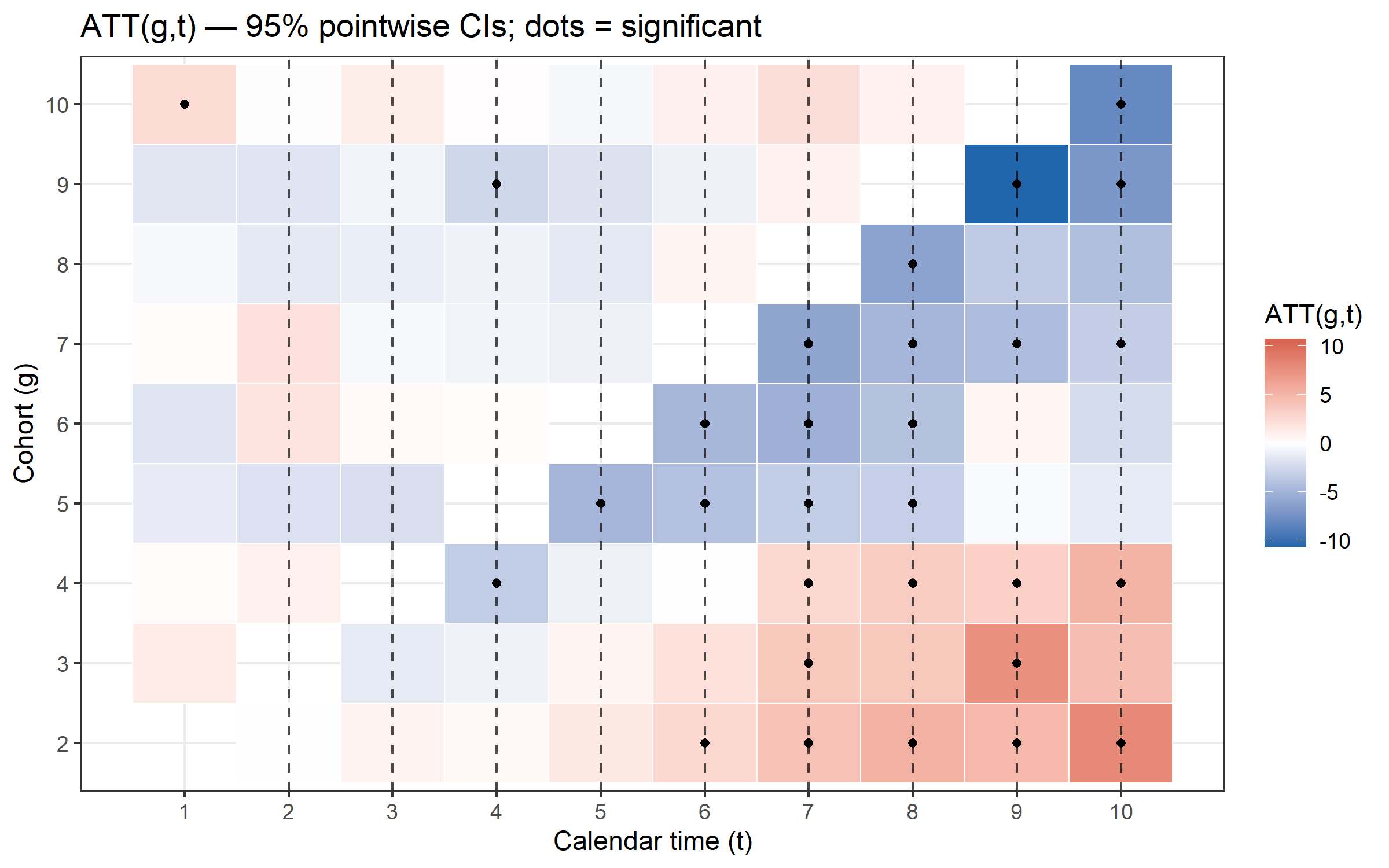
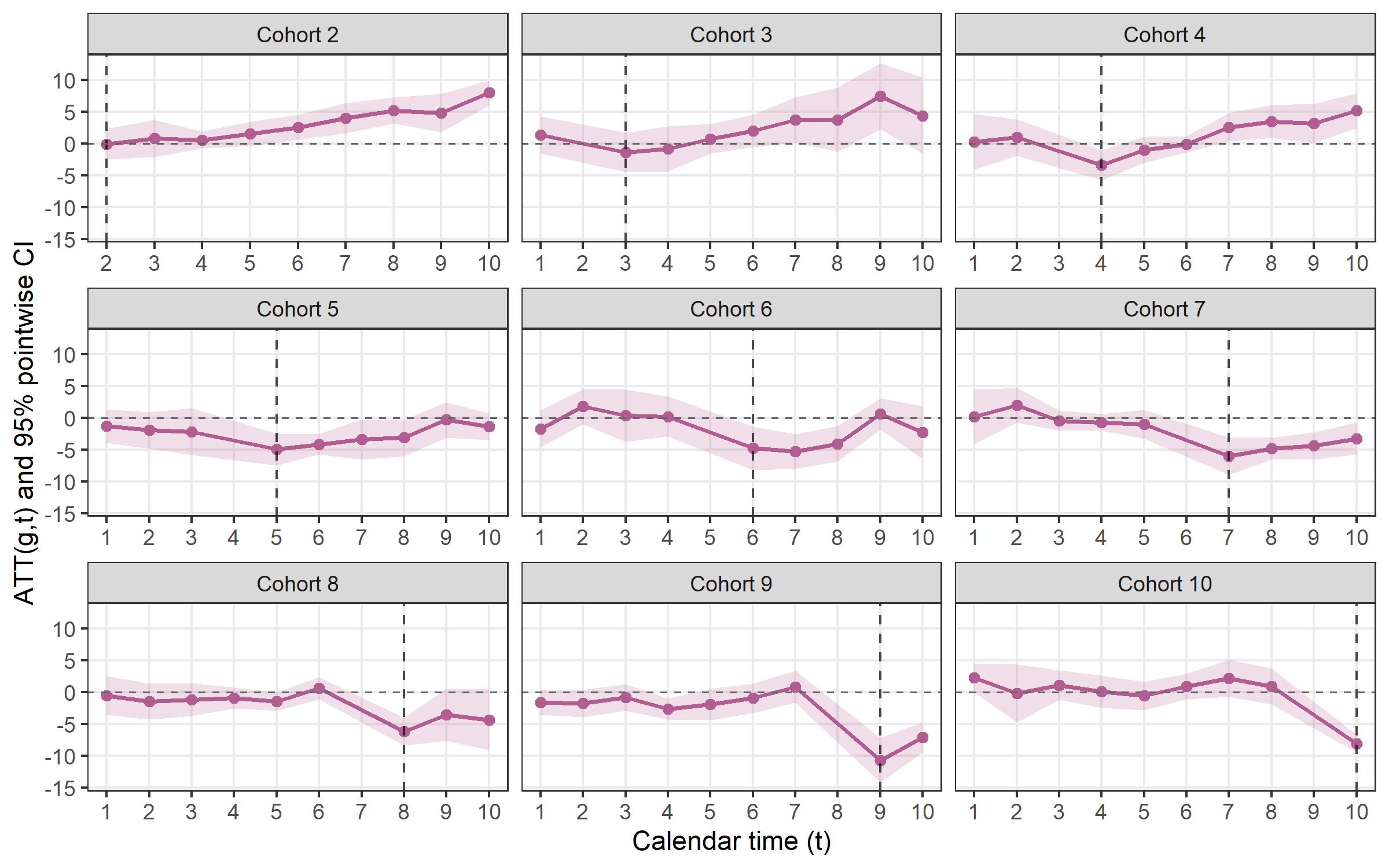
plot(flex)

---

ATT aggregation — att()

After estimating event_study() with a staggered estimator, att() computes a single aggregated ATT — or one per cohort / per calendar period.

# Overall ATT
att_simple <- att(
  data        = df_stagg,
  outcome     = y,
  time        = year,
  timing      = timing,
  unit        = id,
  estimator   = "cs",
  aggregation = "simple"
)

print(att_simple)

## ATT Estimation  [estimator: CS | aggregation: Simple (overall)]
## N = 950 obs | 95 units | 45 treated
## 
##   group estimate std.error statistic  p.value conf_low_95 conf_high_95
## 1    NA   -0.755     0.226     -3.35 0.000813        -1.2       -0.313

# Per-cohort ATT
att(df_stagg, y, year, timing, unit = id,
         estimator = "cs", aggregation = "by_cohort")

# Per-calendar-period ATT
att(df_stagg, y, year, timing, unit = id,
         estimator = "cs", aggregation = "by_time")

Supported estimators for att(): "cs" (Callaway-Sant’Anna 2021) and "bjs" (Borusyak et al. 2024).

---

Bootstrap simultaneous confidence bands

Pointwise CIs control error rates one period at a time. When you plot 15 pre- and post-treatment estimates, the joint false-positive rate may exceed 5 %. Simultaneous bands (Callaway & Sant’Anna 2021, Corollary 1) provide joint coverage across the entire event-study curve.

cs_boot <- event_study(
  data          = df_stagg,
  outcome       = y,
  time          = year,
  timing        = timing,
  unit          = id,
  staggered     = TRUE,
  estimator     = "cs",
  control_group = "nevertreated",
  bootstrap     = TRUE,
  boot_reps     = 999,
  boot_seed     = 42
)

# Lighter outer band = simultaneous CI; darker inner band = pointwise CI
plot(cs_boot, show_simultaneous = TRUE)

plot(cs_boot, interactive = TRUE, show_simultaneous = TRUE)

---

Honest sensitivity analysis — honest_sensitivity()

Event-study estimates rely on the parallel trends assumption. Rather than testing pre-trends and hoping for the best, honest_sensitivity() implements Rambachan & Roth (2023): it reports confidence sets for a post-treatment effect under progressively weaker restrictions on how different post-treatment violations of parallel trends can be from the pre-trends, plus a breakdown value — the largest violation at which the effect is still significant.

res <- event_study(df, outcome = y, treatment = treat, time = year, timing = 6,
              fe = ~ id + year)

# Relative-magnitude restriction: post violation <= Mbar x max pre violation
h <- honest_sensitivity(res, type = "relative_magnitude",
                        m_grid = c(0, 0.5, 1, 1.5, 2))
print(h)          # robust CIs per Mbar + the original (parallel-trends) CI
plot(h)    # "top-down" sensitivity plot

Use type = "smoothness" for the (bounded second difference) restriction. Inference uses the Andrews-Roth-Pakes conditional test — a pure-R reimplementation validated against the HonestDiD package. For estimators other than "twfe", pass betahat and sigma directly. The numeric helpers (lpSolveAPI, Rglpk, TruncatedNormal, Matrix, pracma) are optional Suggests.

---

Plotting options

plot() works with results from any estimator.

plot(es, type = "errorbar")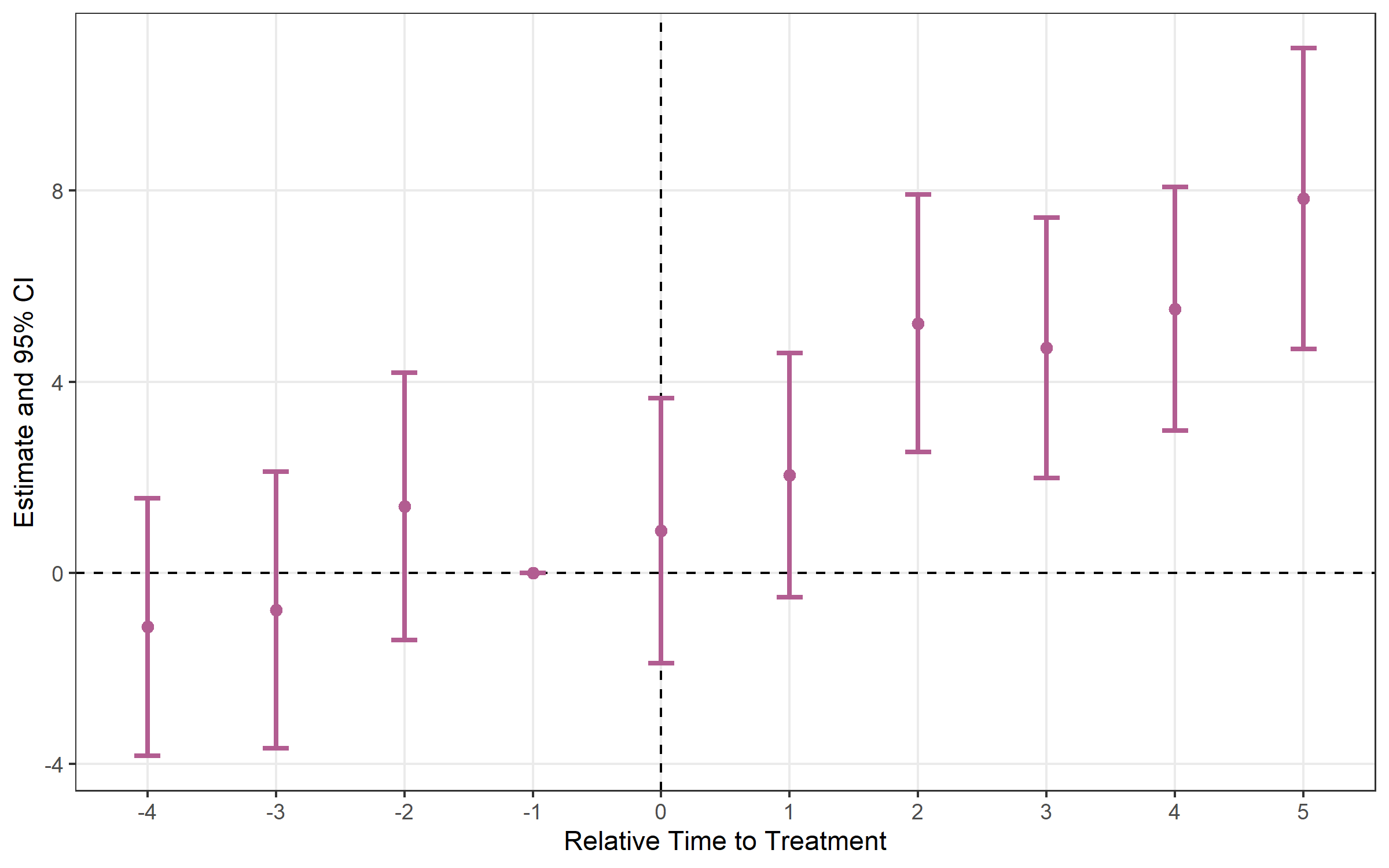

es_multi <- event_study(
  data      = df,
  outcome   = y,
  treatment = treat,
  time      = period,
  timing    = 5,
  fe        = ~ id + period,
  cluster   = ~ id,
  conf_level = c(0.90, 0.95, 0.99)
)
plot(es_multi, ci_level = 0.90, theme_style = "minimal")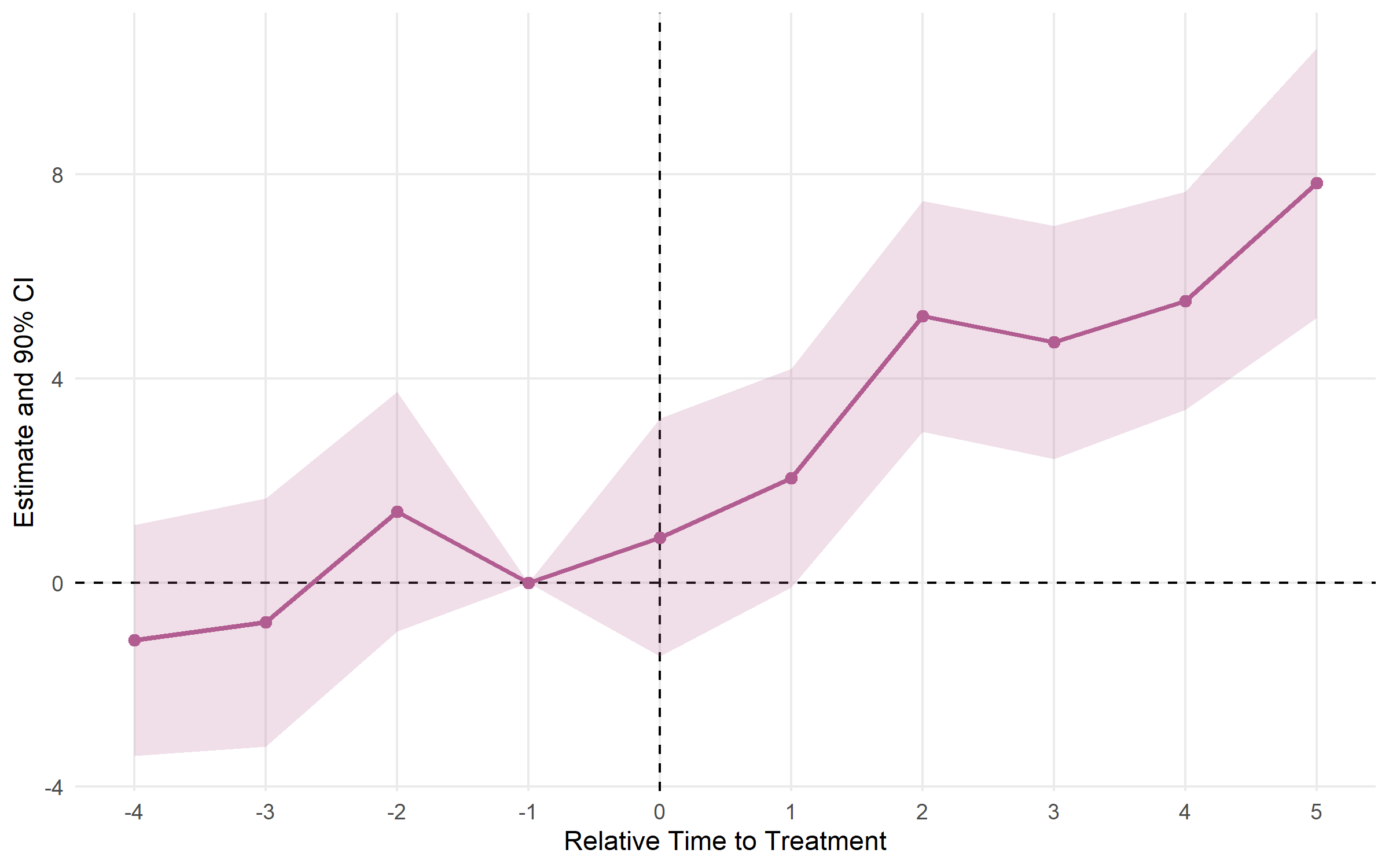

Interactive plots

plot(es, interactive = TRUE)

---

Key arguments

did()

Argument	Default	Description
data	—	Data frame (panel)
outcome	—	Outcome variable (unquoted; expressions like log(y) OK)
treatment	—	Binary D_it indicator, or group dummy when timing is set
timing	NULL	Scalar treatment period; auto-constructs D_it = treatment*(time>=timing)
fe	NULL	FE formula ~ id + year; auto-inferred from unit + time if omitted
unit	NULL	Unit identifier (for FE inference and sample-size metadata)
time	NULL	Time variable (for FE inference and timing-based D_it construction)
covariates	NULL	Additional controls, e.g. ~ x1 + x2
cluster	NULL	Clustering: formula ~ id, column name, or vector
conf_level	0.95	CI level(s); vector allowed
vcov	"HC1"	VCOV type; cluster-robust SE used automatically when cluster is set

event_study()

Argument	Default	Description
data	—	Data frame (panel or RCS)
outcome	—	Outcome variable (unquoted)
treatment	NULL	0/1 treatment dummy ("twfe" only)
time	—	Time variable (numeric)
timing	—	Treatment date (scalar for "twfe", column for others; NA = never treated)
unit	NULL	Unit ID (required for "cs", "sa", "bjs", "twm")
fe	NULL	Fixed effects formula, e.g. ~ id + year
estimator	"twfe"	"twfe", "cs", "sa", "bjs", "twm", or "flex"
staggered	NULL	Inferred: timing naming a column means staggered; override with TRUE/FALSE
group	NULL	FLEX only: treatment group identifier
trends	FALSE	TWM only: cohort-specific linear trends
covariates	NULL	Controls (supported for "twm" and "flex")
control_group	"nevertreated"	CS only: "nevertreated" or "notyettreated"
cluster	NULL	Clustering formula, e.g. ~ id
baseline	-1	Reference period
conf_level	0.95	CI level(s); vector allowed
vcov	"HC1"	VCOV type
bootstrap	FALSE	CS only: multiplier bootstrap for simultaneous CIs
boot_reps	999	Bootstrap draws
boot_seed	NULL	Bootstrap RNG seed

att()

Argument	Default	Description
data	—	Data frame (panel)
outcome	—	Outcome variable (unquoted)
time	—	Calendar time variable
timing	—	First treatment period per unit; NA = never treated
unit	—	Unit identifier (required)
estimator	"cs"	"cs" or "bjs"
aggregation	"simple"	"simple", "by_cohort", or "by_time"
control_group	"nevertreated"	CS only
conf_level	0.95	CI level(s)

---

Contributing

Found a bug or have a feature request? Open an issue on GitHub.